SOM-08-03 Chapter 08 · Columns and Struts

Rankine-Gordon Formula & Eccentrically Loaded Columns

Subject
Strength of Materials (Solid Mechanics)
Chapter
Columns and Struts
Standard Exam Coverage
GATE CE, UPSC ESE, SSC JE, State AE/JE, RRB JE

1. Engineering Context & Overview

While Euler's formula governs long, slender columns failing by pure elastic buckling (λ>89\lambda > 89 for mild steel) and direct crushing governs stubby pedestals (λ<32\lambda < 32), the vast majority of practical civil engineering compression members fall squarely in the intermediate range (32≤λ≤12032 \le \lambda \le 120). In this intermediate regime, failure occurs through a complex interaction of material plastic yielding and geometric flexural instability.

Furthermore, real-world columns are almost never subjected to mathematically concentric axial loads. Beams framing into columns, fabrication tolerances, initial crookedness (e0e_0), and connection eccentricities introduce simultaneous axial force and bending moment.

To address these real-world realities, two monumental theoretical formulations were developed:

  1. The Rankine-Gordon Empirical Formula: An elegant reciprocal formulation that bridges the gap between pure material crushing and pure elastic buckling, valid across all slenderness ratios.
  2. The Secant Formula: An exact analytical derivation that accounts for the non-linear second-order lateral deflection (P−ΔP-\Delta effect) caused by an eccentric compressive load.

Mastering both formulations is essential for competitive examinations (GATE CE, UPSC ESE, SSC JE, State AE) and practical structural design.


2. The Intermediate Column Dilemma & The Rankine Principle

2.1 The Intermediate Gap

Consider the two theoretical extremes of compression failure:

  1. Short Column Failure: Governed purely by the material ultimate compressive crushing strength: Pc=σc⋅AP_c = \sigma_c \cdot A
  2. Long Column Failure: Governed purely by Euler's elastic flexural buckling load: Pe=π2EILe2=π2EAλ2P_e = \frac{\pi^2 E I}{L_e^2} = \frac{\pi^2 E A}{\lambda^2}

In intermediate columns, testing shows that the actual failure load PP is strictly less than both the crushing load PcP_c and the Euler load PeP_e:

Pactual<min⁡(Pc,Pe)P_{\text{actual}} < \min(P_c, P_e)

2.2 The Reciprocal Hypothesis

William John Macquorn Rankine (1820–1872) proposed an empirical reciprocal formulation combining both crushing and buckling resistances:

1PR=1Pc+1Pe\frac{1}{P_R} = \frac{1}{P_c} + \frac{1}{P_e}

where PRP_R is the Rankine Crippling (or Buckling) Load.


3. Mathematical Derivation of the Rankine-Gordon Formula

Starting from the reciprocal equation:

1PR=1Pc+1Pe=Pe+PcPc⋅Pe\frac{1}{P_R} = \frac{1}{P_c} + \frac{1}{P_e} = \frac{P_e + P_c}{P_c \cdot P_e}

Inverting both sides:

PR=Pc⋅PePc+Pe=Pc1+PcPeP_R = \frac{P_c \cdot P_e}{P_c + P_e} = \frac{P_c}{1 + \frac{P_c}{P_e}}

Substitute the analytical expressions for Pc=σc⋅AP_c = \sigma_c \cdot A and Pe=π2EAλ2P_e = \frac{\pi^2 E A}{\lambda^2}:

PcPe=σc⋅Aπ2E⋅Aλ2=(σcπ2E)λ2\frac{P_c}{P_e} = \frac{\sigma_c \cdot A}{\frac{\pi^2 E \cdot A}{\lambda^2}} = \left( \frac{\sigma_c}{\pi^2 E} \right) \lambda^2

Define the Rankine Constant (aa):

a=σcπ2Ea = \frac{\sigma_c}{\pi^2 E}

Substituting this into the equation yields the classical Rankine-Gordon Formula:

PR=σc⋅A1+aλ2=σc⋅A1+a(Lermin⁡)2P_R = \frac{\sigma_c \cdot A}{1 + a \lambda^2} = \frac{\sigma_c \cdot A}{1 + a \left( \frac{L_e}{r_{\min}} \right)^2}

Dividing by the cross-sectional area AA gives the Rankine Crippling Stress (σR\sigma_R):

σR=PRA=σc1+aλ2\sigma_R = \frac{P_R}{A} = \frac{\sigma_c}{1 + a \lambda^2}

3.3 Asymptotic Verification of the Formula

  1. Case 1: Very Short Column (λ→0\lambda \to 0): aλ2→0  ⟹  PR→σcA1+0=σcA=Pca \lambda^2 \to 0 \implies P_R \to \frac{\sigma_c A}{1 + 0} = \sigma_c A = P_c The formula perfectly reproduces the pure material crushing capacity.
  2. Case 2: Very Slender Column (λ→∞\lambda \to \infty): aλ2≫1  ⟹  PR≈σcAaλ2=σcA(σcπ2E)λ2=π2EAλ2=Pea \lambda^2 \gg 1 \implies P_R \approx \frac{\sigma_c A}{a \lambda^2} = \frac{\sigma_c A}{\left( \frac{\sigma_c}{\pi^2 E} \right) \lambda^2} = \frac{\pi^2 E A}{\lambda^2} = P_e The formula smoothly merges into Euler's elastic buckling load.

Because the reciprocal sum 1PR=1Pc+1Pe\frac{1}{P_R} = \frac{1}{P_c} + \frac{1}{P_e} always produces a result smaller than either individual term, the Rankine-Gordon formula provides a smooth, continuous, and universally conservative prediction across the entire spectrum of slenderness ratios (0≤λ≤∞0 \le \lambda \le \infty).


4. Empirical Constants for Engineering Materials

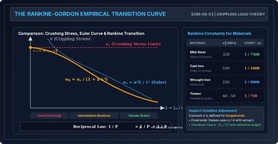
While theoretical a=σcπ2Ea = \frac{\sigma_c}{\pi^2 E}, practical testing shows that material imperfections and residual stresses alter the curvature. Consequently, engineering handbooks and standard codes adopt empirically calibrated values of σc\sigma_c and aa (established for hinged ends):

Material Crushing Stress (σc\sigma_c) Rankine Constant (aa) for Hinged Ends Theoretical λc=1/a\lambda_c = 1/\sqrt{a}
Mild Steel 320 MPa320\text{ MPa} 17500\frac{1}{7500} ≈86.6\approx 86.6
Cast Iron 550 MPa550\text{ MPa} 11600\frac{1}{1600} ≈40.0\approx 40.0
Wrought Iron 250 MPa250\text{ MPa} 19000\frac{1}{9000} ≈94.9\approx 94.9
Structural Timber 40−50 MPa40 - 50\text{ MPa} 1750\frac{1}{750} ≈27.4\approx 27.4
Aluminum Alloy 200 MPa200\text{ MPa} 15000\frac{1}{5000} ≈70.7\approx 70.7

4.1 Adjusting Rankine's Constant for Different End Conditions

The standard Rankine constant aa listed in tables is defined for a hinged-hinged column (Le=LL_e = L). If the column has different end conditions:

  • Best Practice: Always use the universal effective length formulation: PR=σc⋅A1+a(Ler)2P_R = \frac{\sigma_c \cdot A}{1 + a \left( \frac{L_e}{r} \right)^2}
  • Alternative Textbook Notation (using actual length LL):
    • Hinged - Hinged (Le=LL_e = L): Denominator is 1+a(L/r)21 + a (L/r)^2.
    • Fixed - Fixed (Le=L/2L_e = L/2): Denominator is 1+a4(L/r)21 + \frac{a}{4} (L/r)^2.
    • Fixed - Hinged (Le=L/2L_e = L/\sqrt{2}): Denominator is 1+a2(L/r)21 + \frac{a}{2} (L/r)^2.
    • Fixed - Free (Le=2LL_e = 2L): Denominator is 1+4a(L/r)21 + 4a (L/r)^2.

5. Eccentrically Loaded Columns & Derivation of the Secant Formula

In structural reality, loads are rarely concentric. Consider a pinned-pinned column of length LL subjected to an axial compressive load PP acting at an eccentricity ee from the centroidal axis.

      P (Eccentric Load)
      ▼  e
     ──┬── (Top Hinge)
       │
       │\
       │ \
       │  ) δ_max (Mid-Height Lateral Deflection)
       │ /
       │/
     ──┴── (Bottom Hinge)
      ▲  e
      P

5.1 Governing Differential Equation

Choose coordinate origin at the mid-height of the column (x=0x = 0 at mid-height, x=±L/2x = \pm L/2 at the ends). Let y(x)y(x) be the lateral deflection of the centroidal axis from its initial position:

  • At any cross-section xx, the total distance from the line of action of load PP to the deflected centroid is e+y(x)e + y(x).
  • The internal bending moment is: M(x)=−P[e+y(x)]M(x) = -P [e + y(x)]

Equating to flexural curvature:

EId2ydx2=−P[e+y(x)]  ⟹  d2ydx2+k2y=−k2eEI \frac{d^2 y}{dx^2} = -P [e + y(x)] \implies \frac{d^2 y}{dx^2} + k^2 y = -k^2 e

where k2=PEIk^2 = \frac{P}{EI}.

5.2 General Solution & Boundary Conditions

The general solution to this non-homogeneous ODE is:

y(x)=C1cos⁡(kx)+C2sin⁡(kx)−ey(x) = C_1 \cos(kx) + C_2 \sin(kx) - e

Apply the boundary conditions:

  1. Symmetry at Mid-Height (x=0x = 0):

    dydx∣x=0=0  ⟹  −kC1sin⁡(0)+kC2cos⁡(0)=0  ⟹  C2=0\left. \frac{dy}{dx} \right|_{x=0} = 0 \implies -k C_1 \sin(0) + k C_2 \cos(0) = 0 \implies C_2 = 0

    Therefore:

    y(x)=C1cos⁡(kx)−ey(x) = C_1 \cos(kx) - e
  2. Zero Deflection at Ends (x=±L/2x = \pm L/2):

    y(L2)=0  ⟹  C1cos⁡(kL2)−e=0  ⟹  C1=ecos⁡(kL/2)=esec⁡(kL2)y\left(\frac{L}{2}\right) = 0 \implies C_1 \cos\left( \frac{k L}{2} \right) - e = 0 \implies C_1 = \frac{e}{\cos(k L / 2)} = e \sec\left( \frac{k L}{2} \right)

Thus, the deflected shape is:

y(x)=e[cos⁡(kx)cos⁡(kL/2)−1]y(x) = e \left[ \frac{\cos(kx)}{\cos(k L / 2)} - 1 \right]

5.3 Maximum Deflection & Maximum Bending Moment

The maximum lateral deflection occurs at the mid-height (x=0x = 0):

δmax⁡=y(0)=e[sec⁡(kL2)−1]\delta_{\max} = y(0) = e \left[ \sec\left( \frac{k L}{2} \right) - 1 \right]

The maximum bending moment in the column also occurs at mid-height:

Mmax⁡=P(e+δmax⁡)=P(e+e[sec⁡(kL2)−1])M_{\max} = P (e + \delta_{\max}) = P \left( e + e \left[ \sec\left(\frac{k L}{2}\right) - 1 \right] \right) Mmax⁡=P⋅e⋅sec⁡(kL2)M_{\max} = P \cdot e \cdot \sec\left( \frac{k L}{2} \right)

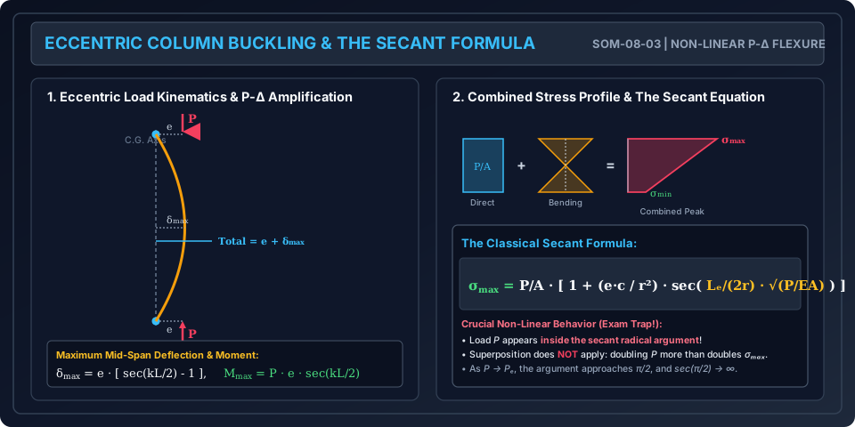
Physical Insight (P−ΔP-\Delta Amplification): In elementary mechanics, the bending moment due to an eccentric load is simply M=P⋅eM = P \cdot e. However, due to lateral deflection of the column, the bending moment is magnified by the factor sec⁡(kL/2)\sec(k L / 2)! This magnification factor approaches infinity as kL/2→π/2k L / 2 \to \pi / 2 (which corresponds to P→PeP \to P_e).


5.4 The Secant Formula for Peak Stress

The maximum compressive stress σmax⁡\sigma_{\max} occurs at the extreme concave fiber at mid-height:

σmax⁡=σdirect+σbending=PA+Mmax⁡⋅cI\sigma_{\max} = \sigma_{\text{direct}} + \sigma_{\text{bending}} = \frac{P}{A} + \frac{M_{\max} \cdot c}{I}

where:

  • cc = Distance from the neutral axis to the extreme compression fiber (c=D/2c = D/2 or d/2d/2).
  • I=A⋅r2I = A \cdot r^2.

Substitute Mmax⁡=Pesec⁡(kL/2)M_{\max} = P e \sec(k L / 2):

σmax⁡=PA+Pesec⁡(kL/2)⋅cAr2=PA[1+e⋅cr2sec⁡(kL2)]\sigma_{\max} = \frac{P}{A} + \frac{P e \sec(k L / 2) \cdot c}{A r^2} = \frac{P}{A} \left[ 1 + \frac{e \cdot c}{r^2} \sec\left( \frac{k L}{2} \right) \right]

Express kk in terms of slenderness ratio:

kL2=L2PEI=L2PEAr2=Le2rPEA=λ2σavgE\frac{k L}{2} = \frac{L}{2} \sqrt{\frac{P}{EI}} = \frac{L}{2} \sqrt{\frac{P}{E A r^2}} = \frac{L_e}{2 r} \sqrt{\frac{P}{E A}} = \frac{\lambda}{2} \sqrt{\frac{\sigma_{\text{avg}}}{E}}

This yields the world-famous Secant Formula:

σmax⁡=PA[1+(e⋅cr2)sec⁡(Le2rPEA)]\sigma_{\max} = \frac{P}{A} \left[ 1 + \left( \frac{e \cdot c}{r^2} \right) \sec\left( \frac{L_e}{2 r} \sqrt{\frac{P}{E A}} \right) \right]

6. Non-Linearity & The Failure of Superposition in Beam-Columns

The Secant Formula reveals a profound departure from elementary beam theory:

  1. Non-Linear Load-Stress Relationship: The applied load PP appears both outside and inside the radical argument of the secant function.
  2. Failure of the Principle of Superposition: If the compressive load PP is doubled, the peak stress σmax⁡\sigma_{\max} more than doubles: σmax⁡(2P)≫2⋅σmax⁡(P)\sigma_{\max}(2P) \gg 2 \cdot \sigma_{\max}(P)
  3. Design Implication: In sizing an eccentric column to an allowable stress σallow\sigma_{\text{allow}}, one cannot simply apply a factor of safety to the stress. The factor of safety (FOSFOS) must be applied to the load PP directly (Pdesign=FOS×PserviceP_{\text{design}} = FOS \times P_{\text{service}}), and the resulting maximum stress must not exceed the yield stress σy\sigma_y.

7. Engineering Diagrams & Visual Walkthrough

Figure 1: The Rankine-Gordon Transition Curve & Empirical Constants

The following diagram illustrates how the Rankine-Gordon empirical curve seamlessly bridges the crushing stress threshold σc\sigma_c and the asymptotic Euler hyperbola, along with the empirical material constant table.

Rankine Gordon Curve Transition

Figure 2: Eccentric Column Kinematics & The Secant Formula

The following diagram details the second-order P−ΔP-\Delta amplification mechanism, the combined direct and flexural stress distribution across the cross-section, and the structure of the Secant Formula.

Eccentric Column Secant Formula

8. Worked Numerical Examples

Example 1: Rankine Crippling Load of a Hollow Cast Iron Column

Problem Statement: A hollow cast iron column of outside diameter Do=200 mmD_o = 200\text{ mm} and inside diameter Di=150 mmD_i = 150\text{ mm} is 5.0 m5.0\text{ m} long with both ends rigidly fixed (Le=0.5L=2.5 mL_e = 0.5 L = 2.5\text{ m}).
Given:

  • Compressive crushing strength: σc=550 MPa\sigma_c = 550\text{ MPa}
  • Rankine's constant for hinged ends: a=11600a = \frac{1}{1600}
  • Modulus of Elasticity: E=100 GPaE = 100\text{ GPa}
  • Factor of safety: FOS=3.0FOS = 3.0
  1. Calculate the Rankine crippling load PRP_R.
  2. Calculate the Euler critical load PeP_e.
  3. Compare the Rankine load with both the pure crushing load PcP_c and the Euler load PeP_e.
  4. Determine the safe working load PsafeP_{\text{safe}}.

Solution:

Step 1: Cross-Sectional Geometric Properties:

  • Cross-sectional Area AA: A=π4(Do2−Di2)=π4[(0.200)2−(0.150)2]=π4[0.0400−0.0225]=0.013744 m2=137.44 cm2A = \frac{\pi}{4} (D_o^2 - D_i^2) = \frac{\pi}{4} \left[ (0.200)^2 - (0.150)^2 \right] = \frac{\pi}{4} [0.0400 - 0.0225] = 0.013744\text{ m}^2 = \mathbf{137.44\text{ cm}^2}
  • Moment of Inertia II: I=π64(Do4−Di4)=π64[(0.200)4−(0.150)4]=π64[1.600×10⁻³−0.50625×10⁻³]I = \frac{\pi}{64} (D_o^4 - D_i^4) = \frac{\pi}{64} \left[ (0.200)^4 - (0.150)^4 \right] = \frac{\pi}{64} [1.600 \times 10^{-3} - 0.50625 \times 10^{-3}] I=π×1.09375×10−364=5.36893×10⁻⁵ m4=5368.93 cm4I = \frac{\pi \times 1.09375 \times 10^{-3}}{64} = 5.36893 \times 10^{-5}\text{ m}^4 = \mathbf{5368.93\text{ cm}^4}
  • Radius of Gyration rr: r=IA=5.36893×10−50.013744=0.06250 m=62.50 mmr = \sqrt{\frac{I}{A}} = \sqrt{\frac{5.36893 \times 10^{-5}}{0.013744}} = \mathbf{0.06250\text{ m}} = \mathbf{62.50\text{ mm}} (Alternatively: r=Do2+Di24=0.0400+0.02254=0.2504=0.0625 mr = \frac{\sqrt{D_o^2 + D_i^2}}{4} = \frac{\sqrt{0.0400 + 0.0225}}{4} = \frac{0.250}{4} = 0.0625\text{ m})

Step 2: Effective Length & Slenderness Ratio: Since both ends are fixed:

Le=0.5×L=0.5×5.0 m=2.50 mL_e = 0.5 \times L = 0.5 \times 5.0\text{ m} = \mathbf{2.50\text{ m}} λ=Ler=2.500.0625=40.00\lambda = \frac{L_e}{r} = \frac{2.50}{0.0625} = \mathbf{40.00}

Step 3: Component Loads (PcP_c and PeP_e):

  • Pure Crushing Load: Pc=σc×A=(550×106 N/m2)×0.013744 m2=7559.46 kNP_c = \sigma_c \times A = (550 \times 10^6\text{ N/m}^2) \times 0.013744\text{ m}^2 = \mathbf{7559.46\text{ kN}}
  • Euler Buckling Load: Pe=π2EILe2=π2×(100×109)×(5.36893×10−5)(2.50)2=52,989,2806.25=8478.28 kNP_e = \frac{\pi^2 E I}{L_e^2} = \frac{\pi^2 \times (100 \times 10^9) \times (5.36893 \times 10^{-5})}{(2.50)^2} = \frac{52,989,280}{6.25} = \mathbf{8478.28\text{ kN}}

Step 4: Rankine Crippling Load (PRP_R): Using Rankine's empirical formula with effective length:

PR=σc⋅A1+a(Ler)2=7559.46 kN1+11600(40)2=7559.461+16001600=7559.461+1=7559.462=3779.73 kNP_R = \frac{\sigma_c \cdot A}{1 + a \left( \frac{L_e}{r} \right)^2} = \frac{7559.46\text{ kN}}{1 + \frac{1}{1600} (40)^2} = \frac{7559.46}{1 + \frac{1600}{1600}} = \frac{7559.46}{1 + 1} = \frac{7559.46}{2} = \mathbf{3779.73\text{ kN}}

(Note: Using the theoretical reciprocal relation: PR=Pc⋅PePc+Pe=7559.46×8478.287559.46+8478.28=3996.27 kNP_R = \frac{P_c \cdot P_e}{P_c + P_e} = \frac{7559.46 \times 8478.28}{7559.46 + 8478.28} = 3996.27\text{ kN})


Step 5: Safe Working Load (PsafeP_{\text{safe}}):

Psafe=PRFOS=3779.73 kN3.0=1259.91 kNP_{\text{safe}} = \frac{P_R}{FOS} = \frac{3779.73\text{ kN}}{3.0} = \mathbf{1259.91\text{ kN}}

Key Observation: Because λ=40\lambda = 40 lies in the intermediate zone where crushing and buckling interact strongly, the Rankine crippling load (3780 kN3780\text{ kN}) is less than half of the Euler load (8478 kN8478\text{ kN}). Relying on Euler's formula would have resulted in catastrophic failure!


Example 2: Structural Column Selection Using Rankine's Formula

Problem Statement: A structural steel column of length L=4.5 mL = 4.5\text{ m} with one end fixed and one end hinged (Le=0.707L=3.1815 mL_e = 0.707 L = 3.1815\text{ m}) must support a working axial load W=350 kNW = 350\text{ kN} with a factor of safety FOS=2.5FOS = 2.5 (Required crippling load PR(req)=2.5×350=875 kNP_{R(\text{req})} = 2.5 \times 350 = 875\text{ kN}).
Mild steel properties: σc=320 MPa\sigma_c = 320\text{ MPa}, Rankine constant a=17500a = \frac{1}{7500}.
Two rolled steel sections are available:

  • Trial Section A (ISMB 350): Area A=66.7 cm2A = 66.7\text{ cm}^2, rxx=14.29 cmr_{xx} = 14.29\text{ cm}, ryy=2.84 cmr_{yy} = 2.84\text{ cm}.
  • Trial Section B (ISWB 300 - Wide Flange): Area A=61.3 cm2A = 61.3\text{ cm}^2, rxx=12.87 cmr_{xx} = 12.87\text{ cm}, ryy=4.82 cmr_{yy} = 4.82\text{ cm}.
    Determine which section is safe under the Rankine formula, and compare their material efficiency.

Solution:

The column is unbraced laterally; therefore, buckling is governed by the least radius of gyration (rmin⁡=ryyr_{\min} = r_{yy}).

Trial Section A (ISMB 350):

  • A=66.7 cm2=6670 mm2A = 66.7\text{ cm}^2 = 6670\text{ mm}^2
  • rmin⁡=ryy=2.84 cm=28.4 mmr_{\min} = r_{yy} = 2.84\text{ cm} = 28.4\text{ mm}
  • Slenderness ratio: λA=Lermin⁡=3181.5 mm28.4 mm=112.02\lambda_A = \frac{L_e}{r_{\min}} = \frac{3181.5\text{ mm}}{28.4\text{ mm}} = \mathbf{112.02}
  • Rankine Crippling Load: PR(A)=σc⋅A1+aλA2=(320 N/mm2)×6670 mm21+17500(112.02)2=2,134,400 N1+12,548.57500=2134.40 kN1+1.6731=2134.402.6731=798.42 kNP_{R(A)} = \frac{\sigma_c \cdot A}{1 + a \lambda_A^2} = \frac{(320\text{ N/mm}^2) \times 6670\text{ mm}^2}{1 + \frac{1}{7500} (112.02)^2} = \frac{2,134,400\text{ N}}{1 + \frac{12,548.5}{7500}} = \frac{2134.40\text{ kN}}{1 + 1.6731} = \frac{2134.40}{2.6731} = \mathbf{798.42\text{ kN}}
  • Capacity check: PR(A)=798.42 kN<875.00 kN  ⟹  P_{R(A)} = 798.42\text{ kN} < 875.00\text{ kN} \implies UNSAFE!

Trial Section B (ISWB 300):

  • A=61.3 cm2=6130 mm2A = 61.3\text{ cm}^2 = 6130\text{ mm}^2
  • rmin⁡=ryy=4.82 cm=48.2 mmr_{\min} = r_{yy} = 4.82\text{ cm} = 48.2\text{ mm}
  • Slenderness ratio: λB=Lermin⁡=3181.5 mm48.2 mm=66.01\lambda_B = \frac{L_e}{r_{\min}} = \frac{3181.5\text{ mm}}{48.2\text{ mm}} = \mathbf{66.01}
  • Rankine Crippling Load: PR(B)=σc⋅A1+aλB2=(320 N/mm2)×6130 mm21+17500(66.01)2=1,961,600 N1+4357.37500=1961.60 kN1+0.5810=1961.601.5810=1240.80 kNP_{R(B)} = \frac{\sigma_c \cdot A}{1 + a \lambda_B^2} = \frac{(320\text{ N/mm}^2) \times 6130\text{ mm}^2}{1 + \frac{1}{7500} (66.01)^2} = \frac{1,961,600\text{ N}}{1 + \frac{4357.3}{7500}} = \frac{1961.60\text{ kN}}{1 + 0.5810} = \frac{1961.60}{1.5810} = \mathbf{1240.80\text{ kN}}
  • Capacity check: PR(B)=1240.80 kN≥875.00 kN  ⟹  P_{R(B)} = 1240.80\text{ kN} \ge 875.00\text{ kN} \implies SAFE! (Reserve margin =+41.8%= +41.8\%)

Material Efficiency Comparison:

Weight Saving=66.7−61.366.7×100=8.10%\text{Weight Saving} = \frac{66.7 - 61.3}{66.7} \times 100 = \mathbf{8.10\%} Strength Increase=1240.80−798.42798.42×100=+55.41%\text{Strength Increase} = \frac{1240.80 - 798.42}{798.42} \times 100 = \mathbf{+55.41\%}

Profound Design Takeaway: The wide-flange section (ISWB 300) saves 8.1%8.1\% in steel weight while delivering 55.4%55.4\% more buckling capacity! The wider flanges significantly boost the weak-axis radius of gyration (ryyr_{yy} increased from 28.4 mm28.4\text{ mm} to 48.2 mm48.2\text{ mm}), dramatically slashing the slenderness ratio.


Example 3: Peak Stress in an Eccentric Column via the Secant Formula

Problem Statement: A solid rectangular steel column of width b=100 mmb = 100\text{ mm} and depth h=150 mmh = 150\text{ mm} has a length L=3.0 mL = 3.0\text{ m} and is pinned at both ends (Le=L=3.0 mL_e = L = 3.0\text{ m}).
Material properties: E=200 GPa=200×103 N/mm2E = 200\text{ GPa} = 200 \times 10^3\text{ N/mm}^2.
An axial compressive load P=250 kNP = 250\text{ kN} is applied with an eccentricity e=15 mme = 15\text{ mm} along the symmetry axis, causing bending about the minor axis (b=100 mmb = 100\text{ mm}).

  1. Calculate the maximum mid-height lateral deflection δmax⁡\delta_{\max}.
  2. Calculate the maximum compressive stress σmax⁡\sigma_{\max} using the Secant Formula.
  3. Compare with the elementary linear estimate that ignores lateral deflection amplification.

Solution:

Step 1: Cross-Sectional Geometric Properties:

  • Area: A=b⋅h=100×150=15,000 mm2=0.015 m2A = b \cdot h = 100 \times 150 = 15,000\text{ mm}^2 = 0.015\text{ m}^2.
  • Bending occurs about the minor axis (b=100 mmb = 100\text{ mm}): I=h⋅b312=150×(100)312=12.50×106 mm4=1.25×10⁻⁵ m4I = \frac{h \cdot b^3}{12} = \frac{150 \times (100)^3}{12} = 12.50 \times 10^6\text{ mm}^4 = 1.25 \times 10^{-5}\text{ m}^4
  • Radius of gyration rr: r=b12=1003.4641=28.8675 mm=0.0288675 mr = \frac{b}{\sqrt{12}} = \frac{100}{3.4641} = \mathbf{28.8675\text{ mm}} = 0.0288675\text{ m}
  • Distance to extreme compression fiber: c=b2=1002=50.0 mm=0.050 mc = \frac{b}{2} = \frac{100}{2} = \mathbf{50.0\text{ mm}} = 0.050\text{ m}
  • Eccentricity ratio: e⋅cr2=15×50(28.8675)2=750833.33=0.9000\frac{e \cdot c}{r^2} = \frac{15 \times 50}{(28.8675)^2} = \frac{750}{833.33} = \mathbf{0.9000}

Step 2: Secant Argument & Deflection Calculation:

  • Parameter kk: k=PEI=250×103(200×109)×(1.25×10−5)=250,0002,500,000=0.1000=0.316228 m−1k = \sqrt{\frac{P}{EI}} = \sqrt{\frac{250 \times 10^3}{(200 \times 10^9) \times (1.25 \times 10^{-5})}} = \sqrt{\frac{250,000}{2,500,000}} = \sqrt{0.1000} = \mathbf{0.316228\text{ m}^{-1}}
  • Argument of the secant function: u=kL2=0.316228×3.0 m2=0.47434 radiansu = \frac{k L}{2} = \frac{0.316228 \times 3.0\text{ m}}{2} = \mathbf{0.47434\text{ radians}} u (degrees)=0.47434×180∘π=27.18∘u \text{ (degrees)} = 0.47434 \times \frac{180^\circ}{\pi} = \mathbf{27.18^\circ}
  • Value of sec⁡(u)\sec(u): cos⁡(27.18∘)=0.88958  ⟹  sec⁡(u)=10.88958=1.12413\cos(27.18^\circ) = 0.88958 \implies \sec(u) = \frac{1}{0.88958} = \mathbf{1.12413}

Step 3: Mid-Height Lateral Deflection (δmax⁡\delta_{\max}):

δmax⁡=e[sec⁡(u)−1]=15 mm×[1.12413−1]=15×0.12413=1.862 mm\delta_{\max} = e [\sec(u) - 1] = 15\text{ mm} \times [1.12413 - 1] = 15 \times 0.12413 = \mathbf{1.862\text{ mm}} Total mid-height eccentricity=e+δmax⁡=15+1.862=16.862 mm\text{Total mid-height eccentricity} = e + \delta_{\max} = 15 + 1.862 = \mathbf{16.862\text{ mm}}

Step 4: Maximum Compressive Stress via Secant Formula:

  • Average direct stress: σdirect=PA=250×103 N15,000 mm2=16.67 MPa\sigma_{\text{direct}} = \frac{P}{A} = \frac{250 \times 10^3\text{ N}}{15,000\text{ mm}^2} = \mathbf{16.67\text{ MPa}}
  • Maximum stress: σmax⁡=PA[1+(e⋅cr2)sec⁡(u)]=16.67×[1+0.9000×1.12413]\sigma_{\max} = \frac{P}{A} \left[ 1 + \left( \frac{e \cdot c}{r^2} \right) \sec(u) \right] = 16.67 \times [1 + 0.9000 \times 1.12413] σmax⁡=16.67×[1+1.0117]=16.67×2.0117=33.53 MPa\sigma_{\max} = 16.67 \times [1 + 1.0117] = 16.67 \times 2.0117 = \mathbf{33.53\text{ MPa}}

Step 5: Comparison with Elementary Linear Stress (Ignoring P−ΔP-\Delta):

  • Elementary bending moment: Melem=P×e=250 kN×0.015 m=3.75 kN⋅mM_{\text{elem}} = P \times e = 250\text{ kN} \times 0.015\text{ m} = 3.75\text{ kN}\cdot\text{m}.
  • Elementary bending stress: σb(elem)=Melem⋅cI=(3.75×10⁶ N⋅mm)×50 mm12.50×106 mm4=15.00 MPa\sigma_{b(\text{elem})} = \frac{M_{\text{elem}} \cdot c}{I} = \frac{(3.75 \times 10^6\text{ N}\cdot\text{mm}) \times 50\text{ mm}}{12.50 \times 10^6\text{ mm}^4} = \mathbf{15.00\text{ MPa}}
  • Elementary peak stress: σelem=σdirect+σb(elem)=16.67+15.00=31.67 MPa\sigma_{\text{elem}} = \sigma_{\text{direct}} + \sigma_{b(\text{elem})} = 16.67 + 15.00 = \mathbf{31.67\text{ MPa}}
  • Stress Underestimation: The elementary method underestimates the true flexural stress by a factor equal to sec⁡(u)=1.1241\sec(u) = \mathbf{1.1241} (12.4%12.4\% underestimation of the bending component).

9. Perry-Robertson Formula & Modern Code Formulations

In modern steel structures (IS 800:2007 and Eurocode 3), neither pure Euler nor empirical Rankine is used directly for sizing. Instead, design is based on the Perry-Robertson Formula, which analytically incorporates an initial geometric out-of-straightness e0e_0:

(σy−σ)(σe−σ)=η⋅σe⋅σ(\sigma_y - \sigma)(\sigma_e - \sigma) = \eta \cdot \sigma_e \cdot \sigma

where:

  • σe=π2Eλ2\sigma_e = \frac{\pi^2 E}{\lambda^2} (Euler stress).
  • η=α(λ−0.2)\eta = \alpha (\lambda - 0.2) is the imperfection parameter, with α\alpha representing the imperfection factor for different column buckling classes:
    • Class a (α=0.21\alpha = 0.21): Hot rolled I-sections with thick flanges (highest quality).
    • Class b (α=0.34\alpha = 0.34): Standard rolled I-sections, RHS/SHS hollow tubes.
    • Class c (α=0.49\alpha = 0.49): Standard channels, angles, built-up welded sections.
    • Class d (α=0.76\alpha = 0.76): Heavy welded box sections, thick plates.

10. Common Misconceptions & Exam Pitfalls

[!WARNING] Pitfall 1: Assuming Superposition Holds for Eccentrically Loaded Columns In beams, doubling the lateral load doubles the stress. In columns, doubling the axial load PP increases the secant argument Le2rPEA\frac{L_e}{2r}\sqrt{\frac{P}{EA}}, causing sec⁡(u)\sec(u) to grow rapidly. Stress grows non-linearly. Superposition is completely invalid.

[!CAUTION] Pitfall 2: Neglecting End Restraint in the Rankine Constant The constant a=1/7500a = 1/7500 (mild steel) is strictly for pinned ends. When using actual length LL for a fixed-fixed column, the denominator must use a/4a/4, or simply use the effective length Le=0.5LL_e = 0.5L with the original constant aa.

[!NOTE] Pitfall 3: Inverting the Rankine Reciprocal Expression The formula is 1PR=1Pc+1Pe\frac{1}{P_R} = \frac{1}{P_c} + \frac{1}{P_e}. Some students mistakenly write PR=Pc+PeP_R = P_c + P_e, which gives an absurd load greater than both! Remember: PRP_R is always strictly less than both PcP_c and PeP_e.


11. Real-World Engineering Applications & Standard Codes

  1. Building Column Design in IS 800:2007 (Section 7):
    • Structural steel columns are classified into 4 buckling curves (a,b,c,da, b, c, d) based on cross-section geometry, flange thickness, and residual stresses.
    • Design compressive strength fcd=fy/γm0ϕ+[ϕ2−λ2]0.5f_{cd} = \frac{f_y / \gamma_{m0}}{\phi + [\phi^2 - \lambda^2]^{0.5}}, where ϕ=0.5[1+α(λ−0.2)+λ2]\phi = 0.5 [1 + \alpha(\lambda - 0.2) + \lambda^2].
  2. Reinforced Concrete Columns in IS 456:2000 (Clause 25.1.2):
    • A compression member is classed as "short" when both slenderness ratios Lex/DL_{ex} / D and Ley/bL_{ey} / b are less than 12. If either exceeds 12, it is designed as a slender column with additional second-order moments (P−ΔP-\Delta effects).
  3. Transmission Towers and Trusses:
    • Slender angle sections used as tower diagonals must have their effective length adjusted for bolt end fixity (IS 802 Part 1).
12. Quick Revision Summary & Formula Sheet

Formulation / Parameter Analytical Expression Application / Notes
Rankine Reciprocal Law 1PR=1Pc+1Pe\frac{1}{P_R} = \frac{1}{P_c} + \frac{1}{P_e} Conservative across all λ\lambda
Rankine Crippling Load PR=σc⋅A1+a(Ler)2P_R = \frac{\sigma_c \cdot A}{1 + a \left(\frac{L_e}{r}\right)^2} Standard form for calculations
Rankine Constant (aa) a=σcπ2Ea = \frac{\sigma_c}{\pi^2 E} Mild Steel: 17500\frac{1}{7500}; Cast Iron: 11600\frac{1}{1600}
Rankine Crippling Stress σR=σc1+aλ2\sigma_R = \frac{\sigma_c}{1 + a \lambda^2} Crippling stress in MPa\text{MPa}
Mid-Height Deflection (e≠0e \ne 0) δmax⁡=e[sec⁡(kL2)−1]\delta_{\max} = e \left[ \sec\left(\frac{k L}{2}\right) - 1 \right] Maximum lateral displacement
Mid-Height Moment (e≠0e \ne 0) Mmax⁡=P⋅e⋅sec⁡(kL2)M_{\max} = P \cdot e \cdot \sec\left(\frac{k L}{2}\right) Magnified by P−ΔP-\Delta effect
Secant Formula σmax⁡=PA[1+e⋅cr2sec⁡(Le2rPEA)]\sigma_{\max} = \frac{P}{A} \left[ 1 + \frac{e \cdot c}{r^2} \sec\left( \frac{L_e}{2r} \sqrt{\frac{P}{EA}} \right) \right] Exact peak fiber compressive stress
Eccentricity Ratio e⋅cr2\frac{e \cdot c}{r^2} Dimensionless geometric parameter
Secant Argument (uu) u=Le2rPEAu = \frac{L_e}{2r} \sqrt{\frac{P}{EA}} Must be in radians when computing secant
Perry-Robertson Imperfection η=α(λ−0.2)\eta = \alpha (\lambda - 0.2) Basis of IS 800:2007 column curves