Pure Bending Theory and the Flexure Formula
In this chapter (4 topics)
On this page
- 1. Topic Metadata
- 2. Physical Mechanics & Theoretical Foundation
- 2.1 The Euler-Bernoulli Kinematic Hypothesis
- 2.2 The Neutral Surface and Neutral Axis (NA)
- 3. Mathematical Derivations & Governing Equations
- 3.1 Kinematic Derivation of Longitudinal Fiber Strain ε(y)
- 3.2 Constitutive Equation (Hooke's Law)
- 3.3 Static Equilibrium & Location of the Neutral Axis
- 3.4 Flexural Curvature & Section Modulus
- 4. Engineering Assumptions & Validity Limits
- 5. SVG Technical Illustrations & Diagrammatic Analysis
- Figure 1: Pure Bending Kinematics & Strain Derivation
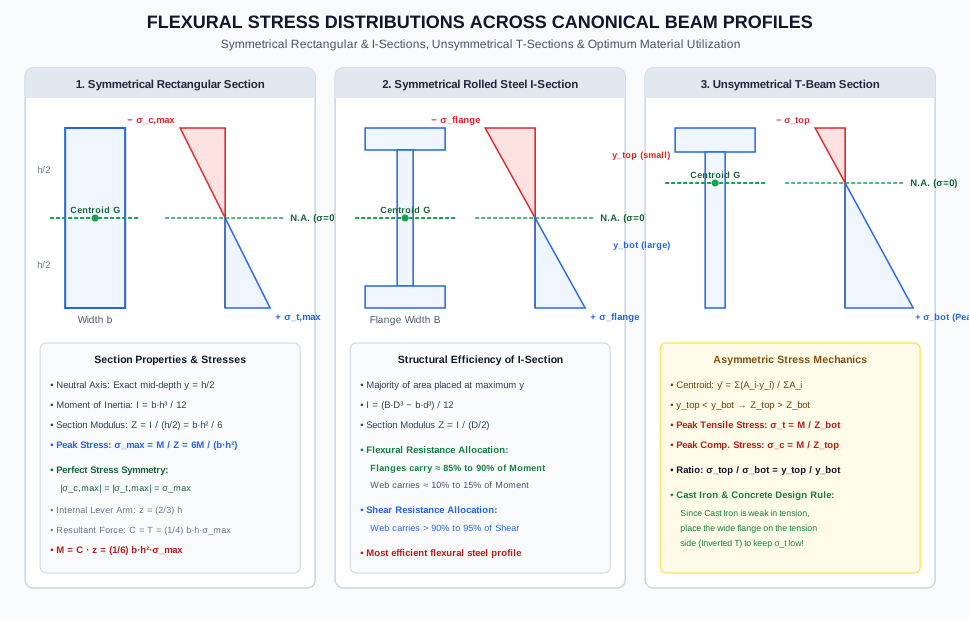
- Figure 2: Flexural Stress Distributions Across Canonical Cross-Sections
- 6. Solved Numerical Examples (Python-Verified)
- Example 1: Sizing and Curvature of a Rectangular Timber Floor Beam
- Example 2: Steel I-Beam (ISMB) — Flange vs Web Moment Allocation
- Example 3: Unsymmetrical Cast Iron T-Beam — Inverted vs Upright Optimization
- 7. Engineering Applications & Real-World Case Studies
- 8. Comparative Analysis & Summary Matrix
- 9. Key Takeaways & Exam-Oriented Mnemonics
- 10. Common Pitfalls, Traps & Misconceptions
- 11. Standard Specifications & Code Provisions
- 12. Comprehensive Formula Box & Practice Problems
- Governing Formula Summary
- Practice Problems
1. Topic Metadata
| Field | Detail |
|---|---|
| Topic Identifier | SOM-04-01 |
| Subject | Strength of Materials / Solid Mechanics |
| Chapter | Bending Stresses in Beams (04_bending_stresses_in_beams) |
| Difficulty Level | Fundamental to Intermediate |
| Target Examinations | GATE CE, UPSC ESE, SSC JE, State AE/JE, RRB JE |
| Primary Prerequisites | Centroid & Moment of Inertia (), Bending Moment Diagrams, Hooke's Law () |
| Governing Equations | , , |
| Authoritative Code References | IS 456:2000, IS 800:2007, IRC:24-2010 |
2. Physical Mechanics & Theoretical Foundation
When a structural beam is subjected to transverse transverse loads, it experiences internal bending moments and shear forces. If a portion of a beam is subjected to a constant bending moment () with zero transverse shear force (), that portion is in a state of pure bending (or simple bending).
         M ↷                                              ↶ M
        ┌───┐============================================┌───┐
        │   │←──────────── Pure Bending Zone ───────────→│   │
        └───┘             (V = 0, M = const)             └───┘
2.1 The Euler-Bernoulli Kinematic Hypothesis
The foundational premise of classical beam theory (developed by Jacob Bernoulli and Leonhard Euler) is the kinematic assumption of plane sections:
"Transverse cross-sections of a beam which are plane and perpendicular to the longitudinal centroidal axis before bending remain plane and perpendicular to the deflected longitudinal axis after bending."
Physical Ramifications of the Hypothesis:
- Absence of Cross-Sectional Warping: The cross-section does not bulge, warp, or distort out-of-plane. Longitudinal displacement varies strictly linearly with depth :
- Zero Transverse Shear Strain (): Because plane sections remain strictly normal to the neutral axis, right angles between the longitudinal fibers and transverse planes remain right angles ().
- Uniaxial Stress State (): Longitudinal beam fibers behave as independent, unconstrained tensile or compressive filaments free to expand or contract laterally according to Poisson's ratio .
2.2 The Neutral Surface and Neutral Axis (NA)
- Neutral Surface: An internal longitudinal physical layer within the beam where longitudinal fibers neither elongate nor contract during bending (strain ).
- Neutral Axis (NA): The line of intersection between the neutral surface and any transverse cross-section.
- In pure elastic flexure, the Neutral Axis must pass through the centroid of the cross-section.
- Fibers located on one side of the NA undergo longitudinal compression (), while fibers on the opposite side undergo longitudinal tension ().
3. Mathematical Derivations & Governing Equations
3.1 Kinematic Derivation of Longitudinal Fiber Strain
Consider an infinitesimal segment of a beam bounded by two initially parallel transverse planes separated by differential length .
Under an applied sagging bending couple , the beam bends into a circular arc of radius subtending a differential angle at the center of curvature :
                             O (Center of Curvature)
                            / \
                           /   \
                          /  dθ \
                         /       \
                 R - y  /         \
                       /           \
               ───────┌─────────────┐─────── Top Face (Compressed)
                      │  Fiber at y │ Arc = (R - y) dθ
               =======╞═════════════╡======= Neutral Surface (Arc = R dθ)
                      │             │
               ───────└─────────────┘─────── Bottom Face (Stretched)
                      |←─── dx ────→|
- Length of the Neutral Fiber: Because the neutral fiber experiences zero strain, its deformed length equals its original undeformed length :
- Length of an Arbitrary Fiber at Distance from the Neutral Axis: Let be measured positive downwards (towards the convex, stretched face):
- Longitudinal Normal Strain :
If is measured positive upwards (towards the concave, compressed face):
Kinematic Conclusion: Longitudinal normal strain varies strictly linearly with perpendicular distance from the neutral axis, irrespective of whether the material is elastic or plastic.
3.2 Constitutive Equation (Hooke's Law)
Assuming the material behaves linearly elastically ():
Because and are constant across any given cross-section:
Kinematic & Constitutive Conclusion: Normal bending stress varies strictly linearly across the cross-sectional depth, vanishing at the neutral axis () and attaining maximum magnitude at the extreme outer fibers ().
3.3 Static Equilibrium & Location of the Neutral Axis
For pure bending, the internal stresses must satisfy two static equilibrium requirements:
Condition 1: Pure Flexural Equilibrium (Zero Net Axial Thrust)
Because there is no external axial load applied ():
Substitute :
Since :
The integral represents the first moment of area of the cross-section about the neutral axis. For the first moment of area to vanish:
Theorem: In linear elastic pure bending, the neutral axis passes precisely through the centroid of the cross-sectional area.
Condition 2: Moment Equilibrium & Derivation of Flexure Formula
The total internal resisting moment developed by normal stresses must equilibrate the applied external bending moment ():
The integral represents the second moment of area (moment of inertia) of the cross-section about the centroidal neutral axis:
Therefore:
Combining this with the constitutive relation yields the celebrated Flexure Formula:
3.4 Flexural Curvature & Section Modulus
1. Flexural Curvature () and Rigidity ()
The curvature is the reciprocal of the radius of curvature :
- Flexural Rigidity (): The product of the material's elastic modulus and the section's second moment of area . It quantifies the beam's resistance to flexural bending distortion.
2. Section Modulus ()
The maximum bending stress occurs at the extreme outer fiber located at maximum distance from the neutral axis:
where:
- For a doubly symmetric section (e.g., rectangle, I-beam, circle), :
- For an unsymmetrical section (e.g., T-section, channel about weak axis), two section moduli exist:
4. Engineering Assumptions & Validity Limits
- Straight Prismatic Beam: The beam is initially straight, and all cross-sections along its length are identical. (Curved beams experience non-linear hyperbolic stress distributions).
- Homogeneous & Isotropic Material: Modulus of elasticity is identical in tension and compression and uniform throughout the cross-section. (Composite/flitched beams require the modular ratio transformation method).
- Hooke's Law Validity: Stresses remain strictly within the proportional limit ().
- Plane Sections Remain Plane: Cross-sections remain planar and undistorted (valid for slender beams with span-to-depth ratio ). Deep beams ( for simply supported, for cantilevers) violate this assumption due to significant shear deformations.
- Radius of Curvature is Large: such that fiber length prior to bending can be taken as .
- Pure Transverse Bending: Applied loads act strictly in a longitudinal plane of symmetry passing through the shear center, preventing coupled torsional twisting or unsymmetrical biaxial bending.
5. SVG Technical Illustrations & Diagrammatic Analysis
Figure 1: Pure Bending Kinematics & Strain Derivation
The following technical diagram demonstrates the circular arc geometry of a differential beam segment undergoing pure flexure, showing radial lines subtending angle , the unextended neutral axis, and the resulting linear strain and normal stress profiles.
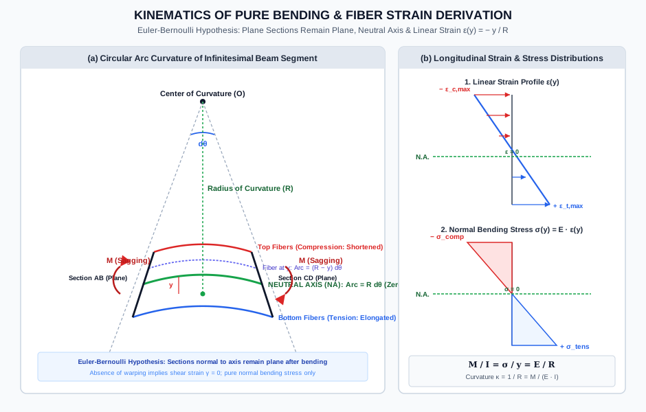
Figure 2: Flexural Stress Distributions Across Canonical Cross-Sections
The following diagram contrasts the linear flexural stress distribution across symmetrical rectangular sections, rolled steel I-sections (highlighting flange moment concentration), and unsymmetrical T-sections (highlighting unequal peak stresses).
6. Solved Numerical Examples (Python-Verified)
Example 1: Sizing and Curvature of a Rectangular Timber Floor Beam
Problem Statement: A simply supported rectangular timber beam of span supports a uniformly distributed dead plus live load of (including self-weight) and a central concentrated load from a partition post. The beam has a cross-section of width and depth . The elastic modulus of timber is .
Determine:
- The maximum bending moment in the beam.
- The centroidal moment of inertia and section modulus .
- The peak flexural compressive and tensile stresses .
- The radius of curvature of the beam's neutral axis at the midspan section.
- The normal stress and strain at a fiber located above the neutral axis.
       w = 6 kN/m                       W = 15 kN (at midspan)
     ↓↓↓↓↓↓↓↓↓↓↓↓↓↓↓↓↓↓↓↓↓↓↓↓↓↓↓↓↓↓↓↓        ↓
   ▲=========================================▲
   A (x = 0)                              B (x = 5 m)
                   b = 150 mm, h = 300 mm
Solution:
Step 1: Calculate Maximum Bending Moment : By loading and support symmetry, the maximum bending moment occurs at midspan ():
Step 2: Cross-Sectional Geometric Properties: For a solid rectangular cross-section:
Step 3: Extreme Fiber Bending Stresses: Applying the flexure formula:
- Top extreme fiber (): Compressive stress .
- Bottom extreme fiber (): Tensile stress .
Step 4: Radius of Curvature at Midspan: From :
Curvature of the beam:
Step 5: Stress and Strain at Fiber Above NA: Because stress and strain vary strictly linearly:
Longitudinal strain:
Example 2: Steel I-Beam (ISMB) — Flange vs Web Moment Allocation
Problem Statement: A symmetrical rolled steel I-beam has the following cross-sectional dimensions:
- Flange width
- Flange thickness
- Web thickness
- Overall depth (clear web depth )
The beam is subjected to a sagging bending moment .
- Calculate the total moment of inertia about the neutral axis.
- Determine the peak bending stress in the extreme flange fibers and the stress at the web-flange junction.
- Calculate the exact percentage of the total bending moment carried by the flanges versus the web.
Solution:
Step 1: Moment of Inertia Calculation: Using the subtraction method (outer bounding rectangle minus the two void spaces):
Step 2: Extreme Fiber and Junction Stresses:
- Extreme Outer Fiber ():
- Web-Flange Junction ():
Step 3: Moment Contribution of Web vs Flanges: The moment of inertia of the web alone about the neutral axis:
Moment of inertia contributed by the two flanges:
Because curvature is common to both components:
Structural Engineering Finding: The flanges constitute only of the cross-sectional area, yet they resist of the bending moment!
Example 3: Unsymmetrical Cast Iron T-Beam — Inverted vs Upright Optimization
Problem Statement: A Cast Iron beam is designed with a T-cross-section having the following dimensions:
- Flange: wide thick.
- Web: thick deep.
- Total depth .
Cast iron has unequal permissible stresses due to its brittle crystalline structure:
- Permissible tensile stress:
- Permissible compressive stress: (ratio )
The beam is simply supported and carries a positive (sagging) bending moment. Calculate the safe allowable moment capacity for:
- Configuration A: Upright T-section (flange on top, stem pointing down).
- Configuration B: Inverted T-section (flange at bottom, stem pointing up).
- Compute the percentage increase in flexural load-carrying capacity achieved simply by inverting the beam.
Solution:
Step 1: Centroid and Neutral Axis Location: Measure reference coordinate from the bottom tip of the stem for the upright orientation:
- Web (Area 1): ,
- Flange (Area 2): ,
- Total Area:
Centroid from bottom edge ():
Distance from centroid to top edge ():
Step 2: Moment of Inertia (Parallel Axis Theorem):
Step 3: Configuration A (Upright T-Beam — Flange on Top): Under sagging moment, top fibers are in compression and bottom fibers are in tension:
- Top fiber (compression):
- Bottom fiber (tension):
Moment governed by permissible tension:
Moment governed by permissible compression:
Allowable moment is governed by the smaller value:
Step 4: Configuration B (Inverted T-Beam — Flange at Bottom): Inverting the beam flips the distance to the tension and compression zones:
- Bottom fiber (tension, wide flange):
- Top fiber (compression, stem tip):
Moment governed by permissible tension:
Moment governed by permissible compression:
Allowable moment for Configuration B:
Step 5: Percentage Increase in Capacity:
Key Exam Observation: Inverting the T-section more than doubles the flexural capacity () with zero additional material cost. This exemplifies the critical principle of tailoring cross-sectional geometry to the asymmetric constitutive strengths of brittle materials.
7. Engineering Applications & Real-World Case Studies
- Structural Steel Girder Sizing (IS 800:2007 Cl. 8.2): In rolled steel I-sections (ISMB, ISWB) and built-up plate girders, the section modulus governs elastic design. When bending occurs about the major axis, wide flanges are positioned at maximum distance from the neutral axis to achieve maximum per kilogram of steel.
- Reinforced Concrete T-Beams (IS 456:2000 Cl. 23.1): In monolithic floor slabs, cast-in-place slabs act compositely as the compressive flange of the supporting beams, creating T-beams and L-beams. Because concrete is strong in compression and negligible in tension, placing the slab at the top (compression zone under sagging moments) maximizes flexural efficiency. Over interior supports of continuous beams (where moments hog), the flange is in tension, forcing the rectangular web to resist compression.
- Prestressed Concrete Railroad Ties / Sleepers: Precast concrete ties are designed under flexural curvature equations. Prestressing tendons induce a pre-compression that offsets the tensile flexural stresses created by heavy axle train loads.
- Craneway Runway Rails (ASME B30.2 / IS 3443): Crane rail heads undergo high localized flexural tension at the base of the rail flange. The flexure formula combined with foundation modulus determines the required rail weight (e.g., or ).
8. Comparative Analysis & Summary Matrix
| Beam Cross-Section | Area | Centroid | Moment of Inertia | Section Modulus | Flexural Efficiency Factor |
|---|---|---|---|---|---|
| Solid Rectangle () | |||||
| Solid Circle () | |||||
| Hollow Circle () | (Thin-walled) | ||||
| Diamond / Square on Diagonal () | |||||
| Rolled Steel I-Section | (Highest!) |
9. Key Takeaways & Exam-Oriented Mnemonics
- The Flexure Trinity: :
- Connects applied loading (), section geometry (), material stiffness (), and physical deformation ().
- Cross-Sectional Efficiency Hierarchy:
- Diamond vs Square Trap (Famous ESE Question):
- When a square section of side is bent with sides horizontal: .
- When bent with a diagonal horizontal: .
- A square beam is stronger when placed with its sides horizontal than when placed with a diagonal horizontal!
- Asymmetrical Section Rule:
- For Cast Iron under sagging moment Invert the T-section (wide flange at bottom).
- For Cast Iron under hogging moment Upright T-section (wide flange at top).
10. Common Pitfalls, Traps & Misconceptions
[!WARNING] Pitfall 1: Assuming the Neutral Axis is Always at Mid-Depth The neutral axis passes through the centroid (). For unsymmetrical shapes (T-sections, channels, compound beams), the centroid is NOT at mid-depth. Always compute first before attempting flexure calculations!
[!CAUTION] Pitfall 2: Neglecting the Difference Between and For an unsymmetrical beam, using a single section modulus is incorrect. Stresses at the top and bottom fibers differ in direct proportion to their distances from the centroid (). In brittle materials, the smaller allowable stress does NOT automatically govern until evaluated against the respective !
[!NOTE] Pitfall 3: Misinterpreting in Pure Bending is the radius of curvature of the neutral axis, not the top or bottom fiber. Curvature is . High bending moment produces a small radius of curvature (tight bend).
11. Standard Specifications & Code Provisions
| Standard | Clause / Section | Engineering Requirement |
|---|---|---|
| IS 800:2007 | Table 2 & Cl. 8.2.1.2 | Classification of cross-sections for flexure: Class 1 (Plastic), Class 2 (Compact), Class 3 (Semi-compact), Class 4 (Slender). Bending strength for Class 3 semi-compact sections is limited strictly to the elastic section modulus . |
| IS 456:2000 | Cl. 22.1 & Annex G | Assumptions for flexural design of reinforced concrete beams: plane sections remain plane (), tensile strength of concrete is ignored in flexure, maximum compressive strain in concrete is taken as . |
| IS 456:2000 | Cl. 23.1.2 | Effective flange width for monolithic T-beams: . |
| IRC:24-2010 | Cl. 504.2 | Allowable elastic flexural stress in steel bridge girders: maximum extreme fiber tension and compression limited to under serviceability load combinations. |
12. Comprehensive Formula Box & Practice Problems
Governing Formula Summary
Practice Problems
-
(GATE CE Pattern) A beam of rectangular cross-section is simply supported over a span of . If the maximum allowable bending stress is , find the maximum concentrated central point load that the beam can support.
- Answer: . Moment capacity . For central point load, .
-
(UPSC ESE Pattern) Two beams, one of solid circular cross-section of diameter and another of square cross-section of side , have the same cross-sectional area. The ratio of the section modulus of the square beam to that of the circular beam is:
- Answer: Equal area: . For square beam, . For circular beam, . Ratio . The square beam is stronger in flexure than a circular beam of identical area.
-
(SSC JE Pattern) In a beam subjected to pure bending, the strain at any fiber varies:
- (A) Inversely with distance from neutral axis
- (B) Directly with distance from neutral axis
- (C) Parabolically with depth
- (D) Remains constant throughout
- Answer: (B) Directly with distance from neutral axis ().