Combined Bending, Torsion & Axial Loading on Shafts
In this chapter (3 topics)
On this page
- 1. Topic Metadata & Scope
- 2. Physical Mechanics & Theoretical Foundation
- 2.1 Why Real Transmission Shafts Experience Combined Loading
- 2.2 Identification of the Critical Surface Element
- 3. Mathematical Derivations: Combined Stresses on Circular Shafts
- 3.1 2D Plane Stress Tensor at the Extreme Fiber
- 3.2 Principal Normal Stresses
- 3.3 Maximum In-Plane Shear Stress
- 4. Equivalent Twisting Moment (Te)
- 4.1 Formal Engineering Definition
- 4.2 Derivation
- 4.3 Design Equation for Ductile Shafts (Guest-Tresca Theory)
- 5. Equivalent Bending Moment (Me)
- 5.1 Formal Engineering Definition
- 5.2 Derivation
- 5.3 Design Equation for Brittle Shafts (Rankine Theory)
- 6. Combined Axial Force, Bending, and Torsion
- 6.1 Total Direct Stress along Shaft Axis
- 6.2 Modified Equivalent Bending and Twisting Moments
- 7. Failure Theories Applied to Power Transmission Shafts
- 7.1 Maximum Distortion Energy Theory (von Mises Theory)
- 7.2 Quantitative Comparison of Required Diameters
- 8. SVG Technical Diagrams & Visual Explanations
- 8.1 3D Loading, Critical Stress Element & Mohr's Circle
- 8.2 Failure Theories Interaction Loci & Sizing Comparison
- 9. Step-by-Step Solved Numerical Examples
- Problem 1: Transmission Shaft Design under Combined M and T (GATE CE Pattern)
- Problem 2: Hollow Shaft under Combined Bending, Torsion & Axial Tension (UPSC ESE Pattern)
- Problem 3: Analytical Proof on the Conservatism of Equivalent Moments
- 10. Comparative Analysis & Summary Matrix
- 11. Key Takeaways & Exam-Oriented Highlights
- 12. Common Traps, Pitfalls & Counter-Intuitive Exam Scenarios
- 13. Standard Code Provisions & Objective Practice Problems
- Reference Code Clauses
- Objective Practice Problems
1. Topic Metadata & Scope
| Attribute | Specification |
|---|---|
| Topic ID | SOM-06-03 |
| Chapter | Chapter 06: Torsion of Circular Shafts (06_torsion_of_shafts) |
| Subject | Strength of Materials (Solid Mechanics) |
| Target Examinations | GATE CE, UPSC ESE, SSC JE, State AE, RRB JE |
| Prerequisites | SOM-02-02 (Principal Stresses & Planes), SOM-02-05 (Theories of Elastic Failure), SOM-04-01 (Flexure Formula), SOM-06-01 (Pure Torsion Formula) |
| Authoritative Reference Codes | ASME Code for Transmission Shafting, IS 2494:1994 (V-Belt Drives - Shaft Design Rules), IS 800:2007 Cl. 9 (Combined Forces) |
| Key Terminology | Transmission shaft, combined bending and torsion, direct axial thrust, plane stress element, principal normal stresses (), maximum shear stress (), Equivalent Bending Moment (), Equivalent Twisting Moment (), Rankine theory, Tresca theory, von Mises distortion energy theory |
2. Physical Mechanics & Theoretical Foundation
2.1 Why Real Transmission Shafts Experience Combined Loading
In mechanical power transmission and civil/structural engineering, a rotating or stationary circular shaft is virtually never subjected to pure torsion alone:
- Transverse Loads from Power Transmission Elements:
- Belts and pulleys impart radial tension forces ().
- Meshing spur and helical gears impart tangential forces (), radial separation forces (), and axial thrust forces ().
- Sprockets and chains exert heavy lateral pulls.
- These transverse loads act perpendicular to the shaft axis across bearing spans, generating substantial transverse bending moments () along the shaft.
- Torque Transmission ():
- The shaft simultaneously delivers mechanical power at angular velocity , maintaining a continuous twisting moment ().
- Axial Loads ():
- Helical gears, bevel gears, ship propeller shafts, and turbine shafts impose significant axial tensile or compressive thrusts ().
2.2 Identification of the Critical Surface Element
Consider a solid or hollow circular shaft of outer diameter subjected to combined bending moment (about the horizontal axis) and torque (about the longitudinal axis):
- Bending Stress Distribution:
- The bending stress is zero at the neutral axis ().
- It reaches its maximum tensile value at the topmost fiber ().
- It reaches its maximum compressive value at the bottommost fiber ().
- Torsional Shear Stress Distribution:
- The torsional shear stress is zero at the center line ().
- It is uniformly distributed at its maximum value everywhere along the outermost cylindrical circumference ().
- The Critical Point:
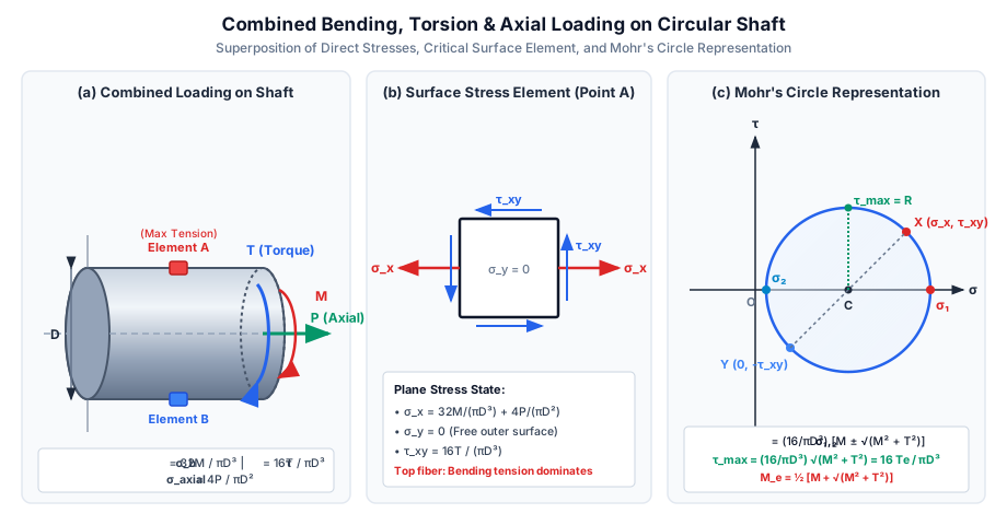
- The critical cross-sectional points are the top and bottom surface fibers where the maximum bending normal stress and maximum torsional shear stress occur simultaneously at the exact same physical coordinates ().
- Because the outer cylindrical surface is exposed to air (free boundary), the radial stress is identically zero:
- Consequently, the material at the extreme fiber is in a state of pure plane stress (2D stress state).
3. Mathematical Derivations: Combined Stresses on Circular Shafts
3.1 2D Plane Stress Tensor at the Extreme Fiber
For a solid circular shaft of diameter :
- Bending Normal Stress:
- Circumferential / Radial Normal Stress:
- Torsional Shear Stress:
The plane stress tensor on the surface element is:
3.2 Principal Normal Stresses
Using the standard 2D transformation formula from SOM-02-02:
Substituting :
Now substitute the expressions for and :
Factoring out the term :
- Major Principal Stress (Maximum Tensile Stress):
- Minor Principal Stress (Maximum Compressive Stress):
Notice that since , the minor principal stress is always negative (compressive) whenever .
3.3 Maximum In-Plane Shear Stress
The maximum shear stress on the surface element is given by the radius of Mohr's circle:
4. Equivalent Twisting Moment ()
4.1 Formal Engineering Definition
Definition: The Equivalent Twisting Moment () is defined as an imaginary, fictitious twisting moment that, if acting alone on the shaft, would produce the same maximum shear stress () as that produced by the combined action of actual bending moment and torque .
4.2 Derivation
- Under pure torque acting alone:
- Under combined bending moment and torque :
- Equating both expressions:
4.3 Design Equation for Ductile Shafts (Guest-Tresca Theory)
According to the Maximum Shear Stress Theory (Tresca / Guest's Theory), yield failure is avoided when the maximum shear stress does not exceed the allowable shear stress :
-
Solid Shaft Sizing:
-
Hollow Shaft Sizing ():
5. Equivalent Bending Moment ()
5.1 Formal Engineering Definition
Definition: The Equivalent Bending Moment () is defined as an imaginary, fictitious bending moment that, if acting alone on the shaft, would produce the same maximum tensile principal stress () as that produced by the combined action of actual bending moment and torque .
5.2 Derivation
- Under pure bending moment acting alone:
- Under combined bending moment and torque :
- Equating both expressions:
Multiplying both sides by :
5.3 Design Equation for Brittle Shafts (Rankine Theory)
According to the Maximum Principal Stress Theory (Rankine's Theory), fracture is avoided when the maximum tensile stress does not exceed the allowable tensile stress :
-
Solid Shaft Sizing:
-
Hollow Shaft Sizing ():
6. Combined Axial Force, Bending, and Torsion
When a shaft transmits an axial thrust force (tension or compression ) in addition to bending moment and torque :
6.1 Total Direct Stress along Shaft Axis
The total normal stress at the outer fiber becomes the algebraic sum of bending stress and axial stress:
- Topmost Fiber (Point A):
- Bottommost Fiber (Point B):
6.2 Modified Equivalent Bending and Twisting Moments
Defining an effective modified bending moment:
The equivalent moments with axial load become:
[!NOTE] For hollow shafts with diameter ratio , the axial stress is , which leads to an effective axial moment term .
7. Failure Theories Applied to Power Transmission Shafts
The choice of design formula depends strictly on the shaft material behavior:
                          Combined Loading on Shaft (M & T)
                                       │
        ┌──────────────────────────────┴──────────────────────────────┐
        ▼                                                             ▼
   Ductile Materials (Mild Steel, Alloy Steel)               Brittle Materials (Cast Iron)
        │                                                             │
        ├─────────────────────────────┐                               ▼
        ▼                             ▼                   Max Principal Stress (Rankine)
Max Shear Stress (Tresca)      Distortion Energy (von Mises)             │
        │                             │                                  ▼
        ▼                             ▼                          σ₁ = 32 M_e / (π D³)
τ_max = 16 T_e / (π D³)      σ_v = 32 M_e,vm / (π D³)                    │
        │                             │                                  ▼
Standard Indian / ASME code      Most accurate, ~15% lighter       M_e = ½ [M + √(M² + T²)]
7.1 Maximum Distortion Energy Theory (von Mises Theory)
For ductile metals, the von Mises equivalent stress under plane stress () is:
Substituting and :
Factoring out :
Hence, the von Mises Equivalent Bending Moment () is:
And the von Mises Equivalent Twisting Moment () is:
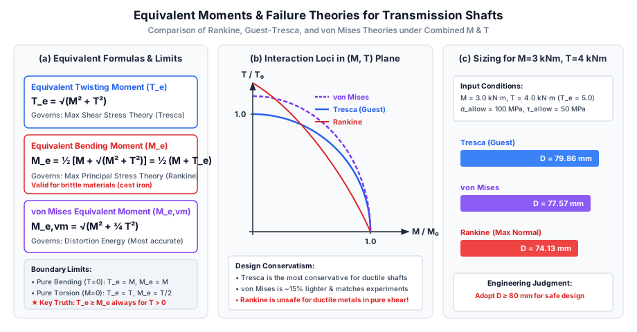
7.2 Quantitative Comparison of Required Diameters
Assume a shaft material where yield strength , Factor of Safety , and :
| Design Theory | Governing Equation | Effective Moment () | Required Diameter |
|---|---|---|---|
| Guest-Tresca (Max Shear) | |||
| von Mises (Distortion Energy) | |||
| Rankine (Max Normal) |
[!WARNING] While Rankine gives the smallest diameter (), Rankine is unsafe for ductile steels! Under pure torsion (), Rankine requires only , underestimating the shear danger by a dangerous factor. For ductile steels, Tresca or von Mises must always be used.
8. SVG Technical Diagrams & Visual Explanations
8.1 3D Loading, Critical Stress Element & Mohr's Circle
The diagram below illustrates the 3D shaft under combined loads, the isolated plane stress square at the top fiber, and the resulting Mohr's circle showing principal stresses and maximum shear stress :
8.2 Failure Theories Interaction Loci & Sizing Comparison
The diagram below presents the mathematical curves for equivalent moments, the normalized interaction loci in the design plane, and the sizing bar chart:
9. Step-by-Step Solved Numerical Examples
Problem 1: Transmission Shaft Design under Combined and (GATE CE Pattern)
Statement:
A solid steel shaft of circular cross-section is subjected to a bending moment and a twisting moment . The material has an allowable tensile stress and an allowable shear stress . Determine:
- The Equivalent Twisting Moment () and Equivalent Bending Moment ().
- The minimum required shaft diameter using the Maximum Shear Stress Theory (Tresca).
- The minimum required shaft diameter using the Maximum Principal Stress Theory (Rankine).
- The percentage difference in required shaft volume between the two theories.
Solution:
Step 1: Calculate Equivalent Moments
- Equivalent Twisting Moment:
- Equivalent Bending Moment:
Step 2: Sizing by Maximum Shear Stress Theory (Tresca)
Step 3: Sizing by Maximum Principal Stress Theory (Rankine)
Step 4: Volume Comparison
Since length is constant, volume is proportional to :
Problem 2: Hollow Shaft under Combined Bending, Torsion & Axial Tension (UPSC ESE Pattern)
Statement:
A hollow circular transmission shaft has an outer diameter and an inner diameter (diameter ratio ). The shaft is subjected simultaneously to:
- A bending moment
- A twisting moment
- An axial tensile force
Calculate:
- The cross-sectional properties ().
- The direct normal stresses due to bending and axial load.
- The principal stresses () and maximum shear stress () at the topmost fiber.
- The principal stresses and maximum shear stress at the bottommost fiber.
Solution:
Step 1: Geometric Properties
- Area:
- Second Moment of Area:
- Elastic Section Modulus:
- Polar Section Modulus:
Step 2: Individual Component Stresses
- Axial Normal Stress (uniform tension across entire cross-section):
- Bending Normal Stress at extreme fiber ():
- Torsional Shear Stress at outer circumference ():
Step 3: Stresses at Topmost Fiber (Point A)
At the top fiber, bending produces tension ():
- Principal Stresses:
- Maximum Shear Stress:
Step 4: Stresses at Bottommost Fiber (Point B)
At the bottom fiber, bending produces compression ():
- Principal Stresses:
- Maximum Shear Stress:
[!TIP] The top fiber is the critical location because tensile axial thrust superimposes constructively with tensile bending stress, raising the peak principal tension to compared to only at the bottom fiber.
Problem 3: Analytical Proof on the Conservatism of Equivalent Moments
Statement:
Prove analytically that for any transmission shaft carrying non-zero bending moment and non-zero torque , the Equivalent Twisting Moment () is strictly greater than the Equivalent Bending Moment (). Furthermore, prove that under equal allowable stresses (), design by Maximum Shear Stress Theory (Tresca) will always yield a strictly larger shaft diameter than design by Maximum Normal Stress Theory (Rankine).
Solution:
Part 1: Proving
By definition:
Subtracting from :
Now examine the term :
Since , we have . Taking the positive square root:
Therefore:
Part 2: Comparison of Required Shaft Diameters
From Tresca's Theory:
Given :
From Rankine's Theory:
Taking the ratio of the two diameters:
Since we proved , the ratio . Therefore:
This rigorously establishes that Tresca's theory is always more conservative than Rankine's theory for power transmission shafts.
10. Comparative Analysis & Summary Matrix
| Parameter / Feature | Equivalent Twisting Moment () | Equivalent Bending Moment () | von Mises Moment () |
|---|---|---|---|
| Governing Failure Theory | Maximum Shear Stress (Guest-Tresca) | Maximum Normal Stress (Rankine) | Distortion Energy (von Mises) |
| Target Material Class | Ductile metals (Mild steel, structural alloys) | Brittle materials (Cast iron, ceramics) | Ductile metals (Best accuracy) |
| Mathematical Expression | |||
| Pure Bending Case () | |||
| Pure Torsion Case () | |||
| Magnitude Hierarchy | Always Largest () | Smallest () | Intermediate () |
| Sizing Equation | |||
| Code Preference | Prescribed by IS 2494 & ASME | Prohibited for ductile transmission | Used in aerospace & advanced piping |
11. Key Takeaways & Exam-Oriented Highlights
- Master Formula for : . It equates maximum shear stress under combined loading to pure torsion.
- Master Formula for : . It equates maximum normal stress to pure bending.
- Pure Torsion Exam Trap: Under pure torsion (), , while . If an exam asks for the equivalent bending moment of a shaft subjected only to torque , the answer is , NOT !
- Pure Bending Exam Trap: Under pure bending (), and .
- Ratio Rule: When , , and .
- von Mises Coefficient: The von Mises equivalent moment is . Note the factor of (or ) multiplying .
- Axial Load Adjustment: When axial thrust acts, simply replace with in both formulas.
12. Common Traps, Pitfalls & Counter-Intuitive Exam Scenarios
- Trap 1: Confusing 16 and 32 in the Sizing Formulas:
Misconception: Using 32 with or 16 with .
Correction: (because ), whereas (because ). Mixing these up results in an incorrect factor of 2 in stress. - Trap 2: Forgetting the Factor in :
Misconception: Writing .
Correction: must be divided by 2: . - Trap 3: Designing Mild Steel Shafts with :
Misconception: Sizing a ductile steel shaft based on and tensile strength.
Correction: Ductile metals fail in shear across slip planes. Sizing by Rankine () is dangerously non-conservative under heavy torque. Sizing must be done using (Tresca) or (von Mises). - Trap 4: Overlooking Minor Principal Stress Sign:
Misconception: Assuming is tensile.
Correction: Since whenever , is strictly negative (compressive). On Mohr's circle, the origin lies between and .
13. Standard Code Provisions & Objective Practice Problems
Reference Code Clauses
- ASME Code for Transmission Shafting:
Prescribes the maximum shear stress design formula including shock and fatigue factors: where is the numerical bending shock factor ( to ) and is the torsional shock factor ( to ). Allowable shear stress is limited to , with an additional reduction if keyways are cut into the shaft. - IS 2494:1994:
Standard provisions for industrial drives; requires transmission shafts to be checked for both strength () and torsional rigidity ().
Objective Practice Problems
Problem 1 (GATE CE)
A solid circular shaft is subjected to a bending moment and a twisting moment . If the maximum normal stress is twice the maximum shear stress (), the ratio of bending moment to twisting moment () is:
- (A)
- (B)
- (C)
- (D) Infinite (pure bending)
Answer: (D)
Solution:
and .
Given :
Squaring both sides: .
Since , (pure bending).
Problem 2 (UPSC ESE)
A circular shaft of diameter is subjected to a twisting moment only (no bending moment). The equivalent bending moment for the shaft is:
- (A)
- (B)
- (C)
- (D)
Answer: (B)
Solution:
Equivalent bending moment is .
For :
.
Problem 3 (SSC JE / RRB JE)
The equivalent twisting moment for a circular shaft subjected to bending moment and twisting moment is given by:
- (A)
- (B)
- (C)
- (D)
Answer: (C)
Solution:
By definition, .
Problem 4 (GATE CE)
A shaft is subjected to simultaneous bending moment and twisting moment . The ratio of maximum shear stress to maximum tensile stress () in the shaft is:
- (A)
- (B)
- (C)
- (D)
Answer: (A)
Solution:
.
.
.
Therefore: .
Problem 5 (State AE / ESE)
According to the Maximum Distortion Energy Theory (von Mises), the equivalent bending moment for a circular shaft under combined bending and torsion is:
- (A)
- (B)
- (C)
- (D)
Answer: (B)
Solution:
.
Equating to yields .