Stress-Strain Behavior of Mild Steel & Brittle Materials
In this chapter (6 topics)
On this page
- 1. Executive Summary & Core Definitions
- 1.1 Key Mechanical Property Definitions
- 2. The Standard Uniaxial Tensile Test (IS 1608 / ISO 6892-1)
- 2.1 Standard Proportional Test Specimen
- 3. Stress-Strain Curve for Structural Mild Steel (Low-Carbon Steel)
- 3.1 Step-by-Step Analysis of Characteristic Points
- 4. Proof Stress & The 0.2% Offset Method
- 4.1 Construction Methodology (IS 1608 / ISO 6892-1)
- 5. Comparative Behavior of Key Civil Engineering Materials
- 6. Failure Modes: Ductile vs Brittle
- 6.1 Ductile Metals (Mild Steel, Copper, Aluminum)
- 6.2 Brittle Materials (Cast Iron, Concrete, Glass)
- 6.3 Behavior Under Uniaxial Compression
- 7. Quantitative Measures of Ductility & Energy Absorption
- 7.1 Percentage Elongation (\% Δ L)
- 7.2 Percentage Reduction in Area (\% Δ A)
- 7.3 Modulus of Resilience (ur)
- 7.4 Modulus of Toughness (ut)
- 8. Indian Standard (IS) Code Specifications
- 8.1 IS 1786:2008 (High Strength Deformed Steel Bars)
- 9. Step-by-Step Solved Numerical Examples
- Example 2.1: Complete Tensile Test Evaluation (UPSC ESE / State AE Level)
- Example 2.2: 0.2% Proof Stress Calculation (GATE CE Level)
- Example 2.3: Modulus of Resilience & Toughness Comparison (GATE / SSC JE)
- 10. Common Pitfalls & Competitive Exam Traps
- 11. Quick Revision Formula Box
- 12. References & Source Literature
1. Executive Summary & Core Definitions
A structural material's capacity to safely bear civil engineering loads depends on its constitutive response under mechanical stress. The standard uniaxial tensile test serves as the universal empirical benchmark for characterizing material elasticity, yield resistance, work hardening, ductility, and fracture toughness.
                                  UNIAXIAL TENSILE TEST
                                            │
                    ┌───────────────────────┴───────────────────────┐
                    ▼                                               ▼
         DUCTILE BEHAVIOR (e.g. Mild Steel)             BRITTLE BEHAVIOR (e.g. Cast Iron, Concrete)
         - Large plastic deformation before fracture.    - Negligible plastic strain before failure.
         - Distinct yield plateau or proof stress.       - Sudden rupture without warning.
         - Fails along 45° maximum shear plane.          - Fails along 90° maximum normal stress plane.
         - Classic "Cup-and-Cone" fracture.              - Flat granular cleavage fracture.
1.1 Key Mechanical Property Definitions
- Ductility: The property of a material enabling it to undergo substantial plastic deformation under tensile load prior to rupture. Quantified by percentage elongation and reduction in area.
- Brittleness: The tendency of a material to fracture under load with little to no prior plastic deformation (elongation at fracture ).
- Malleability: The capacity of a material to undergo extensive plastic deformation under compressive force (hammering, rolling) without cracking.
- Yield Strength (): The stress level at which a material transitions from recoverable elastic behavior to permanent, irrecoverable plastic deformation.
- Ultimate Tensile Strength ( / UTS): The maximum nominal engineering tensile stress the material can sustain before geometric necking instability commences.
- Modulus of Resilience (): The maximum elastic strain energy absorbed per unit volume without permanent deformation (area under the stress-strain curve up to the proportional limit).
- Modulus of Toughness (): The total mechanical energy absorbed per unit volume up to final rupture (entire area under the stress-strain curve).
2. The Standard Uniaxial Tensile Test (IS 1608 / ISO 6892-1)
The tensile test is performed on a Universal Testing Machine (UTM) using standardized cylindrical or flat test coupons.
2.1 Standard Proportional Test Specimen
To ensure test results are independent of specimen dimensions, the initial gauge length () is geometrically proportioned to the original cross-sectional area ( or ) according to the international formula prescribed in IS 1608 (Part 1) / ISO 6892-1:
For a standard cylindrical specimen of circular cross-section with initial diameter :
[!IMPORTANT] In India and British Standard testing, standard round tensile specimens have (e.g., for a standard specimen, gauge length ; for , ). If non-proportional specimens are used, measured percentage elongations cannot be directly compared.
3. Stress-Strain Curve for Structural Mild Steel (Low-Carbon Steel)
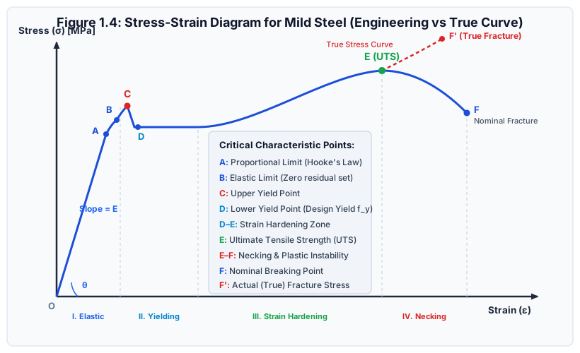
Mild steel (e.g., IS 2062 Grade E250) is the classic structural material exhibiting a pronounced, multi-stage stress-strain curve under tension.
3.1 Step-by-Step Analysis of Characteristic Points
Region OA: Linear Elastic Region
- The curve is a straight line passing through the origin.
- Hooke's Law holds strictly: .
- The slope of line defines Young's Modulus of Elasticity ():
- Point A (Limit of Proportionality): The highest stress level up to which stress remains strictly proportional to strain. For mild steel, .
Point B: Elastic Limit
- The maximum stress the material can sustain without suffering any residual permanent deformation upon complete load removal.
- If unloaded from Point B, the coupon returns along back to zero strain.
- For mild steel, Point B lies very slightly above Point A (). In commercial testing, points A and B are practically coincident.
Point C: Upper Yield Point
- As loading continues past B, elastic resistance breaks down abruptly.
- Microstructural Physics: Interstitial carbon and nitrogen atoms form clusters called Cottrell Atmospheres that anchor dislocations in the iron crystal lattice. At Point C, the applied stress reaches the threshold required to tear dislocations away from these solute pins simultaneously, causing an abrupt drop in the resisting force.
- The upper yield point is sensitive to specimen shape, surface finish, and testing machine loading rate.
Point D: Lower Yield Point
- Once freed from their Cottrell atmospheres, dislocations glide through the crystal lattice at a lower, stable stress level.
- Point D defines the characteristic Yield Strength () of the metal. For standard structural steel, .
- Unlike the upper yield point, the lower yield point is highly stable, reproducible, and insensitive to testing rate. Therefore, all structural design standards (IS 456, IS 800, AISC, Eurocode) base design calculations exclusively on the Lower Yield Stress.
Region D to D': Plastic Yield Plateau (Lüders Bands)
- The specimen elongates significantly (from up to ) under nearly constant stress .
- Visible macroscopic shear deformation bands, called Lüders Bands or Hartmann Lines, propagate along the specimen at angles to the tensile axis.
Region D' to E: Strain Hardening (Work Hardening)
- After the yield plateau, dislocations multiply rapidly, intersect, and form dense tangles, creating a "dislocation forest" that impedes further slip.
- The material regains internal resistance: to produce additional plastic strain, a progressively higher stress must be applied.
- Deformation in this region remains uniform along the entire gauge length (cross-sectional area decreases uniformly).
- Point E (Ultimate Tensile Strength / UTS / ): The peak of the nominal engineering stress-strain curve. For mild steel (E250), .
Region E to F: Necking and Localized Plastic Instability
- At Point E, the rate of strain hardening can no longer keep pace with the geometrical rate of cross-sectional area reduction:
- Deformation ceases to be uniform along the gauge length. Localized plastic thinning (necking) initiates at the weakest cross-section.
- Point F (Nominal Breaking / Fracture Point): The specimen fractures into two pieces. On the nominal engineering curve, the breaking stress at F appears lower than the UTS at E because the load is divided by the original, undeformed area .
Point F' (True Fracture Stress):
- On the true stress-strain curve (where load is divided by the actual instantaneous necked area ), true stress rises continuously to a maximum at final rupture ().
- True fracture stress is significantly higher than both nominal UTS and nominal fracture stress:
4. Proof Stress & The 0.2% Offset Method
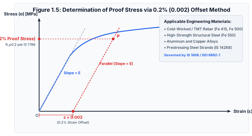
Many modern high-strength structural materials do not display a well-defined yield plateau with upper and lower yield points. Examples include:
- High-Yield Strength Deformed (HYSD / TMT) rebars (Fe 415, Fe 500, Fe 550, Fe 600 per IS 1786).
- Cold-worked and cold-drawn steels.
- Prestressing high-tensile steel strands (IS 14268).
- Aluminum alloys, titanium alloys, and brass.
4.1 Construction Methodology (IS 1608 / ISO 6892-1)
- Plot the accurate experimental engineering stress-strain curve.
- Determine the initial linear elastic slope (Young's modulus).
- On the horizontal strain axis, measure an offset equal to strain ().
- From this offset point, construct a straight line parallel to the linear elastic portion (slope ).
- The point where this parallel line intersects the stress-strain curve is designated as Point .
- The ordinate of Point projected onto the vertical stress axis is defined as the 0.2% Proof Stress ( or ).
[!NOTE] In some specialized non-ferrous specifications (or structural wire ropes), a 0.1% Proof Stress ( with an offset of ) is specified. For structural concrete reinforcement in India, IS 456 and IS 1786 strictly mandate the 0.2% Proof Stress.
5. Comparative Behavior of Key Civil Engineering Materials
STRESS (σ)
  ▲
  │        / High-Strength Alloy Steel (Fe 550)
  │       /   / HYSD / TMT Steel (Fe 415)
  │      /   /   / Mild Steel (Fe 250) [Pronounced yield plateau & necking]
  │     /   /   /
  │    /   /   /────────┐
  │   /   /   /          \
  │  /   /   /            \
  │ │   │   │              x (Ductile Fracture)
  │ │   │   │
  │ │   │   x (Higher strength, reduced ductility)
  │ │   x
  │ │
  │ │ Cast Iron [High compressive strength, brittle tension rupture]
  │ ├──x
  │ │
  │ └───────── Concrete [Low tension, non-linear compression]
  └──────────────────────────────────────────────────────────► STRAIN (ε)
| Material | Behavior Type | Typical Yield / Proof Stress () | Ultimate Tensile Strength () | Fracture Strain () | Characteristic Features |
|---|---|---|---|---|---|
| Mild Steel (Fe 250) | Highly Ductile | Well-defined yield plateau, large elongation, cup-and-cone failure. | |||
| TMT Rebar (Fe 415) | Ductile | Continuous curve; yield determined by 0.2% proof stress. | |||
| TMT Rebar (Fe 500D) | Ductile | 'D' suffix denotes enhanced seismic ductility per IS 1786. | |||
| High Tensile Strand | Moderate Ductility | Used for prestressed concrete; 0.2% proof stress . | |||
| Gray Cast Iron | Highly Brittle | None (No yield) | Very weak in tension; strong in compression (); non-linear. | ||
| Structural Concrete | Brittle | None | (Tension) | Tested in compression (); brittle tensile cracking. | |
| Structural Timber | Orthotropic | Varies by species | (Parallel) | High tensile strength parallel to grain; weak perpendicular to grain. |
6. Failure Modes: Ductile vs Brittle
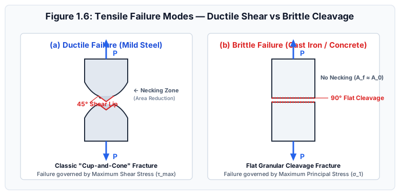
Under uniaxial tensile loading, the macroscopic fracture geometry reflects the underlying microscopic failure criterion:
6.1 Ductile Metals (Mild Steel, Copper, Aluminum)
- Primary Mechanism: Failure is driven by shear slip along planes of maximum shearing stress.
- On an element subjected to uniaxial tensile stress , the maximum shear stress occurs on planes inclined at to the tensile axis:
- Micro-voids coalesce internally at the center of the neck, forming an initial flat crack that propagates outward before shearing off along the shear lip.
- Resulting Fracture Surface: The distinctive "Cup-and-Cone" fracture.
6.2 Brittle Materials (Cast Iron, Concrete, Glass)
- Primary Mechanism: Failure is governed by the Maximum Principal Tensile Stress () overcoming inter-atomic cohesive bonding (cleavage).
- The maximum tensile stress occurs on planes inclined at (i.e., planes oriented at perpendicular to the tensile axis).
- Negligible plastic flow or necking occurs prior to fracture ().
- Resulting Fracture Surface: A flat, rough, granular cleavage plane.
6.3 Behavior Under Uniaxial Compression
- Ductile Materials: Do not fracture in compression. The coupon bulges laterally into a flattened "barrel" shape due to friction at the loading platens, sustaining massive plastic deformation without rupture.
- Brittle Materials (Cast Iron, Concrete): Much stronger in compression than tension. Fail under compression along oblique shear planes inclined at approximately to the horizontal (governed by internal friction per Mohr-Coulomb theory).
7. Quantitative Measures of Ductility & Energy Absorption
7.1 Percentage Elongation ()
where is the original gauge length () and is the final distance between gauge marks after piecing the fractured halves together.
7.2 Percentage Reduction in Area ()
where is the original cross-sectional area and is the minimum necked cross-sectional area measured at the fracture face.
[!TIP] Percentage reduction in area is a truer measure of ductility than percentage elongation because it is localized entirely to the deformation zone and is independent of the initial gauge length.
7.3 Modulus of Resilience ()
The elastic energy absorbed per unit volume up to the elastic limit:
For structural mild steel with and :
7.4 Modulus of Toughness ()
The total mechanical energy absorbed per unit volume up to fracture. Approximated using the trapezoidal rule or empirical formulas:
Mild steel has a much higher modulus of toughness than brittle materials, making it ideal for earthquake-resistant structures that must dissipate seismic kinetic energy through plastic deformation.
8. Indian Standard (IS) Code Specifications
8.1 IS 1786:2008 (High Strength Deformed Steel Bars)
Chemical and mechanical property limits for rebar used in reinforced concrete structures:
| Steel Grade | Minimum Yield / 0.2% Proof Stress (, ) | Minimum Tensile Strength (, ) | Ratio | Minimum % Elongation on |
|---|---|---|---|---|
| Fe 415 | (min ) | |||
| Fe 415D | (min ) | (High ductility) | ||
| Fe 500 | (min ) | |||
| Fe 500D | (min ) | (High ductility) | ||
| Fe 550 | (min ) | |||
| Fe 550D | (min ) | (High ductility) |
Note: As per IS 13920:2016 (Ductile Detailing Code for Seismic Zones III, IV, and V), only 'D' grade rebars (Fe 415D, Fe 500D) satisfying are permitted.
9. Step-by-Step Solved Numerical Examples
Example 2.1: Complete Tensile Test Evaluation (UPSC ESE / State AE Level)
Problem Statement:
A standard cylindrical mild steel coupon of original diameter and gauge length is tested to destruction in a UTM. The following test data are recorded:
- Load at proportional limit:
- Upper yield load:
- Lower yield load:
- Maximum (ultimate) load:
- Breaking (fracture) load:
- Extension at load of (within elastic limit):
- Final gauge length at fracture:
- Diameter at minimum necked section:
Calculate:
- Young's Modulus of Elasticity ().
- Proportional limit stress ().
- Lower yield strength ().
- Ultimate tensile strength ().
- Nominal breaking stress () and True breaking stress ().
- Percentage elongation and percentage reduction in area.
Step-by-Step Solution:
-
Initial Cross-Sectional Area ():
-
Young's Modulus (): Within linear elastic range at with , :
-
Proportional Limit Stress ():
-
Lower Yield Strength ():
-
Ultimate Tensile Strength ():
-
Nominal Breaking Stress vs True Breaking Stress:
- Nominal Breaking Stress:
- Fracture Area ():
- True Breaking Stress:
-
Ductility Parameters:
- Percentage Elongation:
- Percentage Reduction in Area:
Verification Check: Notice that while nominal breaking stress () is lower than UTS (), true breaking stress () is dramatically higher due to the area reduction at the neck.
Example 2.2: 0.2% Proof Stress Calculation (GATE CE Level)
Problem Statement:
A tensile test on an aluminum alloy bar of cross-sectional area and gauge length gives the following load-elongation coordinates in the transition zone:
| Point | Load () | Elongation () | Total Strain | Nominal Stress () |
|---|---|---|---|---|
| 1 | ||||
| 2 | ||||
| 3 | ||||
| 4 | ||||
| 5 | ||||
| 6 |
- Determine the Modulus of Elasticity ().
- Formulate the equation of the 0.2% offset line.
- Determine the 0.2% Proof Stress () of the alloy.
Step-by-Step Solution:
-
Modulus of Elasticity (): Inspecting Points 1, 2, and 3:
Check between Point 2 and 3: . Thus, initial linear elastic modulus .
-
Equation of the 0.2% Offset Line: The offset line begins at on the strain axis with slope :
Rearranging for strain as a function of stress:
-
Finding Intersection with the Experimental Curve:
- At (Point 5): Offset line strain . Experimental strain is (Curve lies above the offset line).
- At (Point 6): Offset line strain . Experimental strain is exactly !
The offset line intersects the experimental curve precisely at Point 6!
Independent Verification Check:
Total strain at Point 6 is .
Elastic strain component: .
Plastic (offset) strain component: (). Exactly verified.
Example 2.3: Modulus of Resilience & Toughness Comparison (GATE / SSC JE)
Problem Statement:
A high-strength alloy steel has yield strength , ultimate strength , and fracture strain . A standard mild steel has , , and fracture strain . Both have .
- Calculate and compare their moduli of resilience ().
- Estimate and compare their moduli of toughness () using the average stress approximation.
Step-by-Step Solution:
-
Modulus of Resilience ():
- High-strength alloy steel:
- Mild steel:
- Comparison: . High-strength steel stores times more recoverable elastic energy (ideal for mechanical springs).
-
Modulus of Toughness ():
- High-strength alloy steel:
- Mild steel:
- Comparison: Despite having less than half the yield strength, mild steel is tougher than the high-strength steel because its higher ductility ( vs ) allows it to absorb far more total energy before complete collapse.
10. Common Pitfalls & Competitive Exam Traps
[!WARNING] Trap 1: The Apparent "Drop" in Breaking Stress
In objective exams, candidates are frequently asked: "At fracture, is the true breaking stress greater than, equal to, or less than the ultimate tensile strength?"
Correct Answer: Greater than!
While the nominal breaking stress is less than the nominal UTS, the true stress (force divided by actual necked area) reaches its absolute maximum at fracture.
[!WARNING] Trap 2: Failure Plane Angle of Cast Iron in Tension vs Compression
In SSC JE and State AE papers:
- Cast iron in tension fails at (flat cleavage plane due to normal stress weakness).
- Cast iron in compression fails along an oblique shear plane () due to shear failure. Confusing tension with compression failure angles is a standard source of lost marks.
[!WARNING] Trap 3: Higher Strength Implies Higher Elastic Modulus
A widespread student misconception: "Higher grade steel (Fe 500) is stiffer than mild steel (Fe 250)."
FALSE! All carbon and low-alloy structural steels share identical Young's Modulus: (). Fe 500 has a higher yield stress, but its initial elastic stiffness is identical to Fe 250.
11. Quick Revision Formula Box
12. References & Source Literature
- Bureau of Indian Standards (2005). IS 1608:2005 / ISO 6892:1998 — Metallic Materials - Tensile Testing at Ambient Temperature, New Delhi.
- Bureau of Indian Standards (2008). IS 1786:2008 — High Strength Deformed Steel Bars and Wires for Concrete Reinforcement (Fourth Revision), New Delhi.
- Dieter, G. E. (1986). Mechanical Metallurgy, 3rd Edition, McGraw-Hill, New York.
- Timoshenko, S. P. (1953). History of Strength of Materials, McGraw-Hill, New York.
- Gere, J. M., & Goodno, B. J. (2018). Mechanics of Materials, 9th Edition, Cengage Learning, Boston.
- Punmia, B. C., Jain, A. K., & Jain, A. K. (2017). Mechanics of Materials, 15th Edition, Laxmi Publications, New Delhi.