SOM-01-05 Chapter 01 · Simple Stresses and Strains

Statically Indeterminate Axially Loaded Systems

In this chapter (6 topics)
On this page
  1. 1. Metadata & Syllabus Mapping
  2. Official Examination Syllabus Mapping
  3. 2. Introduction & Physical Mechanics
  4. The Dual Formulations of Mechanics
  5. 3. Mathematical Formulations & Derivations
  6. 3.1 Prismatic Bar Fixed at Both Ends under an Intermediate Concentrated Load
  7. 3.2 Stepped Bar Fixed at Both Ends
  8. 3.3 Fixed-Fixed Bar under Uniformly Distributed Axial Load
  9. 3.4 Compound / Composite Bars in Parallel (Axial Compression or Tension)
  10. 3.5 Preloaded Fastener Assemblies: Bolt and Sleeve Assembly
  11. 4. Engineering Assumptions & Limitations
  12. 5. Technical Diagrams
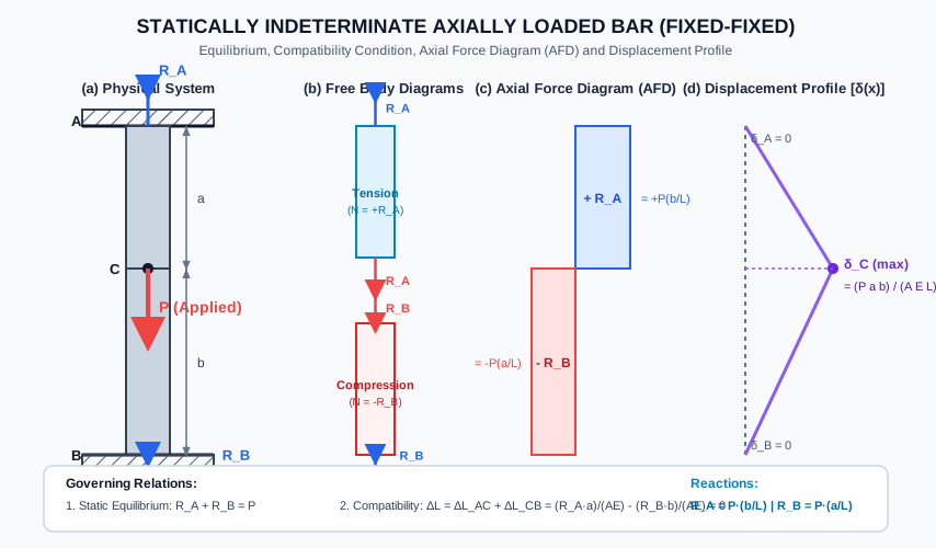
  13. Diagram 1: Fixed-Fixed Bar under Intermediate Axial Load
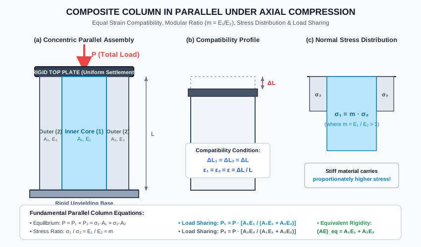
  14. Diagram 2: Concentric Composite Column in Parallel
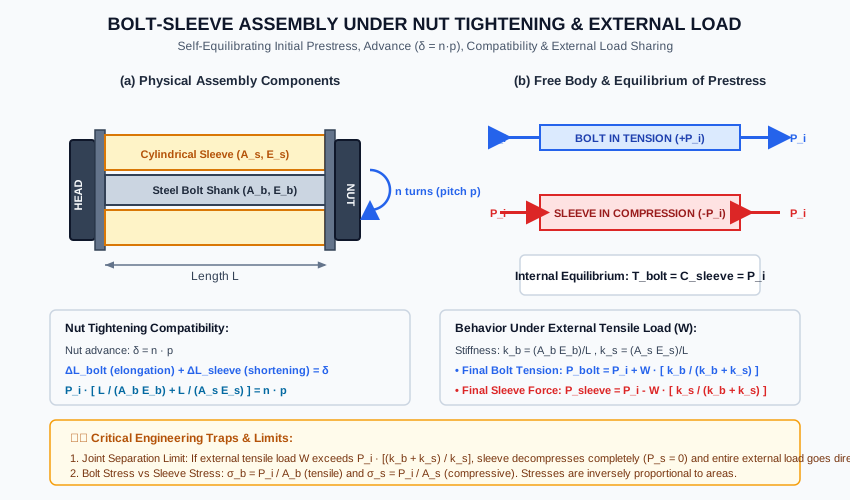
  15. Diagram 3: Bolt-Sleeve Prestress & External Load Assembly
  16. 6. Solved Numerical Examples
  17. Example 5.1: Stepped Bar Fixed at Both Ends under Intermediate Load
  18. Example 5.2: Concentric Composite Column under Axial Load
  19. Example 5.3: Bolt-Sleeve Prestressing and External Tension
  20. 7. Practical Engineering Applications & Field Case Studies
  21. 1. Short Reinforced Concrete Columns (IS 456:2000 Clause 39.3)
  22. 2. High-Strength Friction Grip (HSFG) Preloaded Bolts (IS 800:2007 Clause 10.4)
  23. 3. Structural Jacking and Underpinning
  24. 8. Comparison Tables
  25. Table 1: Statically Determinate vs. Indeterminate Axial Systems
  26. Table 2: Series vs. Parallel Compound Axial Assemblies
  27. 9. Key Engineering Facts & Exam Takeaways
  28. 10. Common Pitfalls, Traps & Anti-Patterns
  29. 11. Standards & Code Provisions
  30. IS 456:2000 (Plain and Reinforced Concrete - Code of Practice)
  31. IS 800:2007 (General Construction in Steel - Code of Practice)
  32. 12. Comprehensive Formula Box & Practice Problems
  33. Master Formula Summary
  34. Practice Problems

1. Metadata & Syllabus Mapping

Attribute Specification
Topic ID SOM-01-05
Module / Subject Subject 02: Strength of Materials (notes/strength_of_materials/)
Chapter Chapter 01: Simple Stresses and Strains (01_simple_stresses_and_strains)
Target Examinations GATE CE, UPSC ESE, SSC JE, RRB JE, State AE, State JE
Prerequisites SOM-01-01 (Stress and Strain), SOM-01-03 (Elastic Constants), SOM-01-04 (Axial Elongation)
Primary Code References IS 456:2000 (Reinforced Concrete Columns), IS 800:2007 (Preloaded HSFG Bolted Joints)
Verification Gate Level 1 through Level 7 Quality Standards

Official Examination Syllabus Mapping

Website note: this mapping is from the author’s notes. It has not been checked against the official notification for each examination; confirm the current syllabus with the examining body.

- GATE Civil Engineering: Solid Mechanics — Statically indeterminate axially loaded members; compound bars and composite sections; modular ratio; displacement compatibility.
- UPSC ESE (Engineering Services): Paper-I Building Materials and Structural Analysis — Compatibility conditions; compound bars; prestressed fasteners and sleeves.
- SSC JE / RRB JE / State AE: Analysis of compound bars; load shared by parallel materials; modular ratio; indeterminate bars fixed at both ends.

2. Introduction & Physical Mechanics

In engineering structural analysis, structural members are classified according to the relationship between the number of unknown reactive forces (rr) and the number of independent equations of static equilibrium (ee):

  1. Statically Determinate Systems: The number of independent equations of static equilibrium is equal to the number of unknown forces (r=er = e). All internal stresses, normal forces, and support reactions can be found strictly using equilibrium:

    ∑Fx=0,∑Fy=0,∑Mz=0\sum F_x = 0, \quad \sum F_y = 0, \quad \sum M_z = 0
  2. Statically Indeterminate Systems: The number of unknown reactions and internal forces exceeds the available equations of static equilibrium (r>er > e). The difference defines the Degree of Static Indeterminacy (DsD_s):

    Ds=r−eD_s = r - e

For an axially loaded straight bar constrained between two unyielding fixed boundaries, there are two unknown support reactions (RAR_A and RBR_B) along the longitudinal axis, but only one non-trivial equation of static equilibrium (∑Fx=0\sum F_x = 0). Hence:

Ds=2−1=1D_s = 2 - 1 = 1

To solve for the unknowns, mechanics requires an additional independent geometric relationship known as the Compatibility Condition (or kinematic constraint).

The Dual Formulations of Mechanics

Formulation Method Primary Unknown Governing Auxiliary Condition
Force Method (Flexibility Method) Redundant Reaction / Internal Force (RR) Geometric deformation / displacement compatibility (ΔL=0\Delta L = 0 or ΔL=δprescribed\Delta L = \delta_{\text{prescribed}})
Displacement Method (Stiffness Method) Nodal Displacements (δi\delta_i) Equilibrium of forces expressed in terms of stiffness coefficients (Kδ=PK \delta = P)

3. Mathematical Formulations & Derivations

3.1 Prismatic Bar Fixed at Both Ends under an Intermediate Concentrated Load

Consider a straight, homogeneous, prismatic bar of length LL, cross-sectional area AA, and Young's modulus EE, rigidly fixed at upper end AA and lower end BB. An intermediate downward axial force PP is applied at point CC, located at distance aa from AA and distance bb from BB (L=a+bL = a + b).

        A (Fixed Support)
        |
        |  Length a, Area A, Modulus E
        |
        * C (Applied downward force P)
        |
        |  Length b, Area A, Modulus E
        |
        B (Fixed Support)

Step 1: Static Equilibrium

Let upward reactive forces at supports AA and BB be RAR_A and RBR_B, respectively.

∑Fy=0  ⟹  RA+RB=P(Eq. 5.1)\sum F_y = 0 \implies R_A + R_B = P \tag{Eq. 5.1}

Step 2: Compatibility Condition

Because ends AA and BB are rigidly anchored to immovable supports, the total change in length between AA and BB must vanish:

ΔLAB=ΔLAC+ΔLCB=0(Eq. 5.2)\Delta L_{AB} = \Delta L_{AC} + \Delta L_{CB} = 0 \tag{Eq. 5.2}

Step 3: Constitutive Relations and Internal Forces

Using section cuts (Free Body Method):

  • In segment ACAC (0≤x≤a0 \le x \le a): The internal axial force is a constant tensile force: NAC=+RA  ⟹  ΔLAC=+RAaAEN_{AC} = +R_A \implies \Delta L_{AC} = +\frac{R_A a}{A E}
  • In segment CBCB (a≤x≤La \le x \le L): The internal axial force is a constant compressive force: NCB=−RB  ⟹  ΔLCB=−RBbAEN_{CB} = -R_B \implies \Delta L_{CB} = -\frac{R_B b}{A E}

Substitute into the compatibility condition:

RAaAE−RBbAE=0  ⟹  RAa=RBb(Eq. 5.3)\frac{R_A a}{A E} - \frac{R_B b}{A E} = 0 \implies R_A a = R_B b \tag{Eq. 5.3}

Step 4: Solution for Support Reactions

Substitute RB=P−RAR_B = P - R_A into Eq. (5.3):

RAa=(P−RA)b=Pb−RAb  ⟹  RA(a+b)=PbR_A a = (P - R_A) b = P b - R_A b \implies R_A (a + b) = P b

Since a+b=La + b = L:

RA=PbL(Eq. 5.4a)\mathbf{R_A = P \frac{b}{L}} \tag{Eq. 5.4a} RB=PaL(Eq. 5.4b)\mathbf{R_B = P \frac{a}{L}} \tag{Eq. 5.4b}

Important Observation: Notice the direct analogy between the axial reactions of a fixed-fixed bar and the transverse reactions of a simply supported beam under a point load! The reaction at either end is directly proportional to the distance of the load from the opposite end.

Step 5: Junction Displacement

The downward displacement of point CC (δC\delta_C) equals the elongation of segment ACAC:

δC=RAaAE=PabAEL(Eq. 5.5)\mathbf{\delta_C = \frac{R_A a}{A E} = \frac{P a b}{A E L}} \tag{Eq. 5.5}

3.2 Stepped Bar Fixed at Both Ends

If the bar comprises nn prismatic segments with lengths LiL_i, cross-sectional areas AiA_i, and elastic moduli EiE_i:

The total compatibility condition remains:

ΔL=∑i=1nNiLiAiEi=0(Eq. 5.6)\Delta L = \sum_{i=1}^n \frac{N_i L_i}{A_i E_i} = 0 \tag{Eq. 5.6}

For a two-segment stepped bar with a load PP applied precisely at the transition shoulder CC:

RAL1A1E1−RBL2A2E2=0  ⟹  RAf1=RBf2(Eq. 5.7)\frac{R_A L_1}{A_1 E_1} - \frac{R_B L_2}{A_2 E_2} = 0 \implies R_A f_1 = R_B f_2 \tag{Eq. 5.7}

where fi=LiAiEif_i = \frac{L_i}{A_i E_i} is the axial flexibility of segment ii.

Combining with equilibrium RA+RB=PR_A + R_B = P:

RA=Pf2f1+f2=PL2A2E2L1A1E1+L2A2E2\mathbf{R_A = P \frac{f_2}{f_1 + f_2} = P \frac{\frac{L_2}{A_2 E_2}}{\frac{L_1}{A_1 E_1} + \frac{L_2}{A_2 E_2}}} RB=Pf1f1+f2=PL1A1E1L1A1E1+L2A2E2\mathbf{R_B = P \frac{f_1}{f_1 + f_2} = P \frac{\frac{L_1}{A_1 E_1}}{\frac{L_1}{A_1 E_1} + \frac{L_2}{A_2 E_2}}}

In terms of axial stiffness ki=1/fi=AiEiLik_i = 1 / f_i = \frac{A_i E_i}{L_i}:

RA=Pk1k1+k2,RB=Pk2k1+k2(Eq. 5.8)\mathbf{R_A = P \frac{k_1}{k_1 + k_2}}, \quad \mathbf{R_B = P \frac{k_2}{k_1 + k_2}} \tag{Eq. 5.8}

3.3 Fixed-Fixed Bar under Uniformly Distributed Axial Load

Consider a prismatic bar of length LL, area AA, and modulus EE, fixed at both ends, subjected to a uniformly distributed downward axial load of intensity qq (force per unit length, N/m or kN/m):

  • By symmetry: RA=RB=qL2(Eq. 5.9)R_A = R_B = \frac{q L}{2} \tag{Eq. 5.9}
  • Internal axial force at distance xx from top support AA: N(x)=RA−qx=qL2−qx=q(L2−x)N(x) = R_A - q x = \frac{q L}{2} - q x = q \left(\frac{L}{2} - x\right)
  • Displacement at any section xx: u(x)=∫0xN(x)AEdx=qAE(Lx2−x22)=qx(L−x)2AE(Eq. 5.10)u(x) = \int_0^x \frac{N(x)}{AE} dx = \frac{q}{AE} \left(\frac{L x}{2} - \frac{x^2}{2}\right) = \frac{q x (L - x)}{2 AE} \tag{Eq. 5.10}
  • Maximum displacement occurs at midspan (x=L/2x = L/2): umax⁡=u(L2)=qL28AE(Eq. 5.11)\mathbf{u_{\max} = u\left(\frac{L}{2}\right) = \frac{q L^2}{8 AE}} \tag{Eq. 5.11}

3.4 Compound / Composite Bars in Parallel (Axial Compression or Tension)

When two or more distinct materials (e.g., concrete core with longitudinal steel rebar, or concentric steel and copper tubes) are bonded together or loaded through a stiff, rigid end plate:

        Rigid Loading Plate  [ |||||| P |||||| ]
        ----------------------------------------
        | Material 1 | Material 2 | Material 1 |
        | (Core / Rebar) | (Matrix / Tube) |
        |   A1, E1   |    A2, E2   |   A1, E1   |
        ----------------------------------------
        Rigid Unyielding Foundation

1. Compatibility Condition

Assuming the end plate remains rigid, both materials undergo identical changes in length:

ΔL1=ΔL2=ΔL(Eq. 5.12)\Delta L_1 = \Delta L_2 = \Delta L \tag{Eq. 5.12}

Since both components share the same original length LL:

ϵ1=ϵ2=ϵ(Eq. 5.13)\epsilon_1 = \epsilon_2 = \epsilon \tag{Eq. 5.13}

2. Constitutive Stress-Strain Relation & Modular Ratio

From Hooke's Law:

σ1=E1ϵ,σ2=E2ϵ\sigma_1 = E_1 \epsilon, \quad \sigma_2 = E_2 \epsilon

Dividing the two equations yields the fundamental stress ratio:

σ1σ2=E1E2=m  ⟹  σ1=m σ2(Eq. 5.14)\mathbf{\frac{\sigma_1}{\sigma_2} = \frac{E_1}{E_2} = m} \implies \mathbf{\sigma_1 = m \, \sigma_2} \tag{Eq. 5.14}

where m=E1E2m = \frac{E_1}{E_2} is the modular ratio.

3. Equilibrium Condition

The total applied force PP is shared between the two materials:

P=P1+P2=σ1A1+σ2A2(Eq. 5.15)P = P_1 + P_2 = \sigma_1 A_1 + \sigma_2 A_2 \tag{Eq. 5.15}

Substitute σ1=mσ2\sigma_1 = m \sigma_2:

P=(mσ2)A1+σ2A2=σ2(mA1+A2)(Eq. 5.16)P = (m \sigma_2) A_1 + \sigma_2 A_2 = \sigma_2 (m A_1 + A_2) \tag{Eq. 5.16}

The term (mA1+A2)(m A_1 + A_2) is defined as the Equivalent Transformed Area in terms of Material 2:

Aeq,2=mA1+A2=E1E2A1+A2(Eq. 5.17)A_{\text{eq}, 2} = m A_1 + A_2 = \frac{E_1}{E_2} A_1 + A_2 \tag{Eq. 5.17}

4. Load Sharing Fractions

Expressing P1P_1 and P2P_2 directly in terms of total load PP:

P1=P[A1E1A1E1+A2E2](Eq. 5.18a)\mathbf{P_1 = P \left[\frac{A_1 E_1}{A_1 E_1 + A_2 E_2}\right]} \tag{Eq. 5.18a} P2=P[A2E2A1E1+A2E2](Eq. 5.18b)\mathbf{P_2 = P \left[\frac{A_2 E_2}{A_1 E_1 + A_2 E_2}\right]} \tag{Eq. 5.18b}

The denominator is the Equivalent Axial Rigidity:

(AE)eq=A1E1+A2E2=∑i=1nAiEi(Eq. 5.19)(AE)_{\text{eq}} = A_1 E_1 + A_2 E_2 = \sum_{i=1}^n A_i E_i \tag{Eq. 5.19}

Total shortening:

ΔL=PL(AE)eq=PLA1E1+A2E2(Eq. 5.20)\mathbf{\Delta L = \frac{P L}{(AE)_{\text{eq}}} = \frac{P L}{A_1 E_1 + A_2 E_2}} \tag{Eq. 5.20}

3.5 Preloaded Fastener Assemblies: Bolt and Sleeve Assembly

A classic structural mechanics assembly consists of a central high-strength steel bolt passed through an outer sleeve (or tube) of a softer material (e.g., bronze, copper, or aluminum) with washers and an end nut.

       [Nut] ===== Washer ===== [Sleeve A_s, E_s] ===== Washer ===== [Bolt Head]
             ================== [Bolt Shank A_b, E_b] ================

Case A: Initial Nut Tightening (Prestress)

Let the nut be turned by nn turns on a thread of pitch pp (mm/turn). The theoretical axial advance of the nut is:

δ=n⋅p(Eq. 5.21)\delta = n \cdot p \tag{Eq. 5.21}

Because the sleeve resists the advance of the nut:

  • The bolt is stretched into tension (T=+PiT = +P_i).
  • The sleeve is squeezed into compression (C=−PiC = -P_i).
  1. Internal Equilibrium: Since no external load is applied to the assembly as a whole:

    ∑Fx=0  ⟹  T=C=Pi(Eq. 5.22)\sum F_x = 0 \implies T = C = P_i \tag{Eq. 5.22}
  2. Deformation Compatibility: The nut advance δ\delta is accommodated partly by the elongation of the bolt (ΔLb\Delta L_b) and partly by the contraction of the sleeve (ΔLs\Delta L_s):

    ΔLb+ΔLs=δ=n⋅p(Eq. 5.23)\Delta L_b + \Delta L_s = \delta = n \cdot p \tag{Eq. 5.23}
  3. Prestress Force Equation:

    PiLbAbEb+PiLsAsEs=n⋅p\frac{P_i L_b}{A_b E_b} + \frac{P_i L_s}{A_s E_s} = n \cdot p

    Assuming equal nominal length Lb≈Ls=LL_b \approx L_s = L:

    PiL[1AbEb+1AsEs]=n⋅pP_i L \left[\frac{1}{A_b E_b} + \frac{1}{A_s E_s}\right] = n \cdot p Pi=n⋅pL[1AbEb+1AsEs]=n⋅p⋅kbkskb+ks(Eq. 5.24)\mathbf{P_i = \frac{n \cdot p}{L \left[\frac{1}{A_b E_b} + \frac{1}{A_s E_s}\right]} = \frac{n \cdot p \cdot k_b k_s}{k_b + k_s}} \tag{Eq. 5.24}

    where kb=AbEbLk_b = \frac{A_b E_b}{L} and ks=AsEsLk_s = \frac{A_s E_s}{L} are the axial stiffnesses of the bolt and sleeve.

  4. Initial Internal Stresses:

    σb=+PiAb(Tensile),σs=−PiAs(Compressive)(Eq. 5.25)\sigma_b = +\frac{P_i}{A_b} \quad (\text{Tensile}), \qquad \sigma_s = -\frac{P_i}{A_s} \quad (\text{Compressive}) \tag{Eq. 5.25}

Case B: Subsequent External Tensile Load WW

Now, suppose an external tensile load WW is applied to the ends of the bolt.

Because the bolt and sleeve are connected in parallel between the washers:

  • The external load increases the elongation of the bolt, thereby increasing its tensile force.
  • The external load relaxes the compressive clamping on the sleeve, thereby decreasing its compressive force.

Let the additional elongation under load WW be ΔLW\Delta L_W:

  • Additional bolt force: ΔPb=+kbΔLW\Delta P_b = +k_b \Delta L_W
  • Sleeve force change: ΔPs=−ksΔLW\Delta P_s = -k_s \Delta L_W

By overall equilibrium:

ΔPb−ΔPs=W  ⟹  (kb+ks)ΔLW=W  ⟹  ΔLW=Wkb+ks\Delta P_b - \Delta P_s = W \implies (k_b + k_s) \Delta L_W = W \implies \Delta L_W = \frac{W}{k_b + k_s}

Therefore:

Pbolt=Pi+W[kbkb+ks](Eq. 5.26a)\mathbf{P_{\text{bolt}} = P_i + W \left[\frac{k_b}{k_b + k_s}\right]} \tag{Eq. 5.26a} Psleeve=Pi−W[kskb+ks](Eq. 5.26b)\mathbf{P_{\text{sleeve}} = P_i - W \left[\frac{k_s}{k_b + k_s}\right]} \tag{Eq. 5.26b}

Joint Separation / Decompression Limit: The sleeve remains compressed (Psleeve>0P_{\text{sleeve}} > 0) only as long as:

W<Wsep=Pi[kb+ksks](Eq. 5.27)W < W_{\text{sep}} = P_i \left[\frac{k_b + k_s}{k_s}\right] \tag{Eq. 5.27}

If W≥WsepW \ge W_{\text{sep}}, the sleeve separates from the washer. The system loses indeterminacy, and the entire external load is carried directly by the bolt: Pbolt=WP_{\text{bolt}} = W.


4. Engineering Assumptions & Limitations

  1. Rigid Plane Assumption: End loading plates and washers are assumed to be infinitely rigid so that cross-sections remain strictly plane, parallel, and experience uniform linear displacement.
  2. Perfect Interface Adhesion: In compound members, the bond between materials is assumed to be 100% monolithic with zero interfacial slip.
  3. Linear Elastic Small Deformations: All materials operate well below their proportional elastic limits (σ≤σprop\sigma \le \sigma_{\text{prop}}), obeying Hooke's Law (E=constantE = \text{constant}).
  4. Prismatic Geometry: Each segment has a uniform cross section and a straight centroidal axis without initial geometric crookedness.
  5. No Elastic Buckling: Under compressive loads, the slenderness ratio is sufficiently low (L/r<30L / r < 30) that axial crushing or elastic instability (Euler buckling) does not precede material yielding.

5. Technical Diagrams

Diagram 1: Fixed-Fixed Bar under Intermediate Axial Load

The following technical vector diagram illustrates the physical system, boundary conditions, free body diagrams of the individual segments, the resulting Axial Force Diagram (AFD), and the linear displacement profile.

Statically Indeterminate Fixed-Fixed Bar

Diagram 2: Concentric Composite Column in Parallel

The vector diagram below shows the equal-strain compatibility condition, modular ratio relation (σ1=mσ2\sigma_1 = m \sigma_2), and load sharing mechanisms for a parallel composite column under axial compression.

Composite Concentric Column in Parallel

Diagram 3: Bolt-Sleeve Prestress & External Load Assembly

The diagram below details the mechanics of nut tightening advance (δ=n⋅p\delta = n \cdot p), the self-equilibrating internal pre-compression and pre-tension, and the subsequent load response under external tensile pulling forces.

Bolt-Sleeve Assembly Tightening and External Load

6. Solved Numerical Examples

Example 5.1: Stepped Bar Fixed at Both Ends under Intermediate Load

A vertical stepped steel bar is rigidly fixed at its upper end AA and lower end BB. The upper segment ACAC has a length of 300 mm300\text{ mm} and a cross-sectional area of 500 mm2500\text{ mm}^2. The lower segment CBCB has a length of 500 mm500\text{ mm} and a cross-sectional area of 250 mm2250\text{ mm}^2. An intermediate downward axial load of 150 kN150\text{ kN} is applied at the junction CC. Taking E=200 GPaE = 200\text{ GPa} throughout:

  1. Determine the reaction forces at supports AA and BB.
  2. Calculate the normal stresses in segments ACAC and CBCB.
  3. Determine the vertical displacement of junction CC.
Given:
Segment 1 (AC): L1 = 300 mm, A1 = 500 mm², E = 200 GPa = 2 × 10⁵ N/mm²
Segment 2 (CB): L2 = 500 mm, A2 = 250 mm², E = 200 GPa = 2 × 10⁵ N/mm²
Applied Load at C: P = 150 kN = 150,000 N (downward)

Solution:

Step 1: Equilibrium Equation
Let RAR_A (upward) and RBR_B (upward) be the reaction forces at supports AA and BB:

∑Fy=0  ⟹  RA+RB=P=150,000 N(i)\sum F_y = 0 \implies R_A + R_B = P = 150{,}000\text{ N} \tag{i}

Step 2: Compatibility Condition
Since supports AA and BB are unyielding:

ΔLAB=ΔLAC+ΔLCB=0\Delta L_{AB} = \Delta L_{AC} + \Delta L_{CB} = 0

Segment ACAC is in tension under upward reaction RAR_A:

ΔLAC=+RAL1A1E\Delta L_{AC} = +\frac{R_A L_1}{A_1 E}

Segment CBCB is in compression under upward reaction RBR_B:

ΔLCB=−RBL2A2E\Delta L_{CB} = -\frac{R_B L_2}{A_2 E}

Therefore:

RAL1A1E−RBL2A2E=0  ⟹  RA(L1A1)=RB(L2A2)(ii)\frac{R_A L_1}{A_1 E} - \frac{R_B L_2}{A_2 E} = 0 \implies R_A \left(\frac{L_1}{A_1}\right) = R_B \left(\frac{L_2}{A_2}\right) \tag{ii}

Step 3: Flexibility Calculation

f1=L1A1=300 mm500 mm2=0.60 mm−1f_1 = \frac{L_1}{A_1} = \frac{300\text{ mm}}{500\text{ mm}^2} = 0.60\text{ mm}^{-1} f2=L2A2=500 mm250 mm2=2.00 mm−1f_2 = \frac{L_2}{A_2} = \frac{500\text{ mm}}{250\text{ mm}^2} = 2.00\text{ mm}^{-1}

From Eq. (ii):

0.60RA=2.00RB  ⟹  RA=2.000.60RB=103RB≈3.3333RB0.60 R_A = 2.00 R_B \implies R_A = \frac{2.00}{0.60} R_B = \frac{10}{3} R_B \approx 3.3333 R_B

Step 4: Solve for Reactions
Substitute into Eq. (i):

(103+1)RB=150,000  ⟹  133RB=150,000\left(\frac{10}{3} + 1\right) R_B = 150{,}000 \implies \frac{13}{3} R_B = 150{,}000 RB=150,000×313=450,00013≈34,615.38 N=34.62 kNR_B = \frac{150{,}000 \times 3}{13} = \frac{450{,}000}{13} \approx \mathbf{34{,}615.38\text{ N} = 34.62\text{ kN}} RA=150,000−34,615.38=1,500,00013≈115,384.62 N=115.38 kNR_A = 150{,}000 - 34{,}615.38 = \frac{1{,}500{,}000}{13} \approx \mathbf{115{,}384.62\text{ N} = 115.38\text{ kN}}

Step 5: Normal Stresses

σAC=+RAA1=115,384.62 N500 mm2=+230.77 MPa(Tension)\sigma_{AC} = +\frac{R_A}{A_1} = \frac{115{,}384.62\text{ N}}{500\text{ mm}^2} = \mathbf{+230.77\text{ MPa} \quad (\text{Tension})} σCB=−RBA2=−34,615.38 N250 mm2=−138.46 MPa(Compression)\sigma_{CB} = -\frac{R_B}{A_2} = -\frac{34{,}615.38\text{ N}}{250\text{ mm}^2} = \mathbf{-138.46\text{ MPa} \quad (\text{Compression})}

Step 6: Displacement of Junction CC
The downward movement of point CC is the elongation of segment ACAC:

δC=ΔLAC=σACL1E=230.77 N/mm2×300 mm2×105 N/mm2=0.3462 mm\delta_C = \Delta L_{AC} = \frac{\sigma_{AC} L_1}{E} = \frac{230.77\text{ N/mm}^2 \times 300\text{ mm}}{2 \times 10^5\text{ N/mm}^2} = \mathbf{0.3462\text{ mm}}

Independent Cross-Check:

δC=∣ΔLCB∣=∣σCB∣L2E=138.46 N/mm2×500 mm2×105 N/mm2=0.3462 mm✓\delta_C = |\Delta L_{CB}| = \frac{|\sigma_{CB}| L_2}{E} = \frac{138.46\text{ N/mm}^2 \times 500\text{ mm}}{2 \times 10^5\text{ N/mm}^2} = 0.3462\text{ mm} \quad \checkmark

Example 5.2: Concentric Composite Column under Axial Load

A short composite column of length L=400 mmL = 400\text{ mm} consists of a solid copper core of diameter d=30 mmd = 30\text{ mm} surrounded by an aluminum alloy tube of inside diameter 30 mm30\text{ mm} and outside diameter 50 mm50\text{ mm}. A total compressive load of P=200 kNP = 200\text{ kN} is applied to the composite column through a rigid top plate. Given Ecopper=100 GPaE_{\text{copper}} = 100\text{ GPa} and Ealuminum=70 GPaE_{\text{aluminum}} = 70\text{ GPa}:

  1. Find the load carried by each material.
  2. Determine the compressive stress in the copper and aluminum.
  3. Compute the total shortening of the column.
Given:
Copper Core: d = 30 mm, E_cu = 100 GPa = 100,000 MPa
Aluminum Tube: d_in = 30 mm, d_out = 50 mm, E_al = 70 GPa = 70,000 MPa
Total Load: P = 200 kN = 200,000 N
Length: L = 400 mm

Solution:

Step 1: Cross-Sectional Areas

Acu=π4d2=π4(30)2=225π≈706.858 mm2A_{\text{cu}} = \frac{\pi}{4} d^2 = \frac{\pi}{4} (30)^2 = 225\pi \approx 706.858\text{ mm}^2 Aal=π4(dout2−din2)=π4(502−302)=π4(2500−900)=400π≈1256.637 mm2A_{\text{al}} = \frac{\pi}{4} (d_{\text{out}}^2 - d_{\text{in}}^2) = \frac{\pi}{4} (50^2 - 30^2) = \frac{\pi}{4} (2500 - 900) = 400\pi \approx 1256.637\text{ mm}^2

Step 2: Axial Rigidities

AcuEcu=706.858 mm2×100,000 N/mm2=7.06858×107 NA_{\text{cu}} E_{\text{cu}} = 706.858\text{ mm}^2 \times 100{,}000\text{ N/mm}^2 = 7.06858 \times 10^7\text{ N} AalEal=1256.637 mm2×70,000 N/mm2=8.79646×107 NA_{\text{al}} E_{\text{al}} = 1256.637\text{ mm}^2 \times 70{,}000\text{ N/mm}^2 = 8.79646 \times 10^7\text{ N}

Total equivalent axial rigidity:

(AE)eq=AcuEcu+AalEal=(7.06858+8.79646)×107=1.58650×10⁸ N(AE)_{\text{eq}} = A_{\text{cu}} E_{\text{cu}} + A_{\text{al}} E_{\text{al}} = (7.06858 + 8.79646) \times 10^7 = 1.58650 \times 10^8\text{ N}

Step 3: Load Sharing

Pcu=P[AcuEcu(AE)eq]=200,000×[7.06858×1071.58650×108]=89,110 N=89.11 kNP_{\text{cu}} = P \left[\frac{A_{\text{cu}} E_{\text{cu}}}{(AE)_{\text{eq}}}\right] = 200{,}000 \times \left[\frac{7.06858 \times 10^7}{1.58650 \times 10^8}\right] = \mathbf{89{,}110\text{ N} = 89.11\text{ kN}} Pal=P[AalEal(AE)eq]=200,000×[8.79646×1071.58650×108]=110,890 N=110.89 kNP_{\text{al}} = P \left[\frac{A_{\text{al}} E_{\text{al}}}{(AE)_{\text{eq}}}\right] = 200{,}000 \times \left[\frac{8.79646 \times 10^7}{1.58650 \times 10^8}\right] = \mathbf{110{,}890\text{ N} = 110.89\text{ kN}}

Sum Check: 89.11 kN+110.89 kN=200.00 kN✓89.11\text{ kN} + 110.89\text{ kN} = 200.00\text{ kN} \quad \checkmark

Step 4: Compressive Stresses

σcu=PcuAcu=89,110 N706.858 mm2=126.06 MPa\sigma_{\text{cu}} = \frac{P_{\text{cu}}}{A_{\text{cu}}} = \frac{89{,}110\text{ N}}{706.858\text{ mm}^2} = \mathbf{126.06\text{ MPa}} σal=PalAal=110,890 N1256.637 mm2=88.24 MPa\sigma_{\text{al}} = \frac{P_{\text{al}}}{A_{\text{al}}} = \frac{110{,}890\text{ N}}{1256.637\text{ mm}^2} = \mathbf{88.24\text{ MPa}}

Modular Ratio Check:

m=EcuEal=100,00070,000=1.4286m = \frac{E_{\text{cu}}}{E_{\text{al}}} = \frac{100{,}000}{70{,}000} = 1.4286 σcuσal=126.0688.24=1.4286=m✓\frac{\sigma_{\text{cu}}}{\sigma_{\text{al}}} = \frac{126.06}{88.24} = 1.4286 = m \quad \checkmark

Step 5: Total Column Shortening

ΔL=PL(AE)eq=200,000 N×400 mm1.58650×108 N=0.5043 mm\Delta L = \frac{P L}{(AE)_{\text{eq}}} = \frac{200{,}000\text{ N} \times 400\text{ mm}}{1.58650 \times 10^8\text{ N}} = \mathbf{0.5043\text{ mm}}

Example 5.3: Bolt-Sleeve Prestressing and External Tension

A high-strength steel bolt of diameter 16 mm16\text{ mm} passes through a bronze sleeve of internal diameter 18 mm18\text{ mm}, external diameter 26 mm26\text{ mm}, and length L=250 mmL = 250\text{ mm}. The nut is initially turned by 1/41/4 of a turn with a thread pitch of 2.0 mm2.0\text{ mm}. Given: Esteel=200 GPaE_{\text{steel}} = 200\text{ GPa}, Ebronze=100 GPaE_{\text{bronze}} = 100\text{ GPa}.

  1. Find the initial pre-tension in the bolt and the initial pre-compression in the sleeve.
  2. Determine the initial stresses in the bolt and sleeve.
  3. If an external tensile load W=30 kNW = 30\text{ kN} is applied to the bolt ends, find the resulting final forces and stresses in both components.
  4. What is the maximum external tensile load that can be applied before the sleeve separates from the washer?
Given:
Steel Bolt: d_b = 16 mm, E_b = 200,000 MPa, L = 250 mm
Bronze Sleeve: d_i = 18 mm, d_o = 26 mm, E_s = 100,000 MPa, L = 250 mm
Nut advance: n = 1/4 turn, pitch p = 2.0 mm ==> delta = 0.25 × 2.0 = 0.50 mm
External Load: W = 30 kN = 30,000 N

Solution:

Step 1: Areas and Component Stiffnesses

Ab=π4(16)2=64π≈201.062 mm2A_b = \frac{\pi}{4} (16)^2 = 64\pi \approx 201.062\text{ mm}^2 As=π4(262−182)=π4(676−324)=88π≈276.460 mm2A_s = \frac{\pi}{4} (26^2 - 18^2) = \frac{\pi}{4} (676 - 324) = 88\pi \approx 276.460\text{ mm}^2

Stiffnesses (k=AELk = \frac{AE}{L}):

kb=201.062×200,000250=160,849.5 N/mm≈1.6085×105 N/mmk_b = \frac{201.062 \times 200{,}000}{250} = 160{,}849.5\text{ N/mm} \approx 1.6085 \times 10^5\text{ N/mm} ks=276.460×100,000250=110,584.1 N/mm≈1.1058×105 N/mmk_s = \frac{276.460 \times 100{,}000}{250} = 110{,}584.1\text{ N/mm} \approx 1.1058 \times 10^5\text{ N/mm} kb+ks=160,849.5+110,584.1=271,433.6 N/mmk_b + k_s = 160{,}849.5 + 110{,}584.1 = 271{,}433.6\text{ N/mm}

Step 2: Initial Prestressing Force (PiP_i)

δ=0.50 mm\delta = 0.50\text{ mm}

Compatibility: ΔLb+ΔLs=δ  ⟹  Pi[1kb+1ks]=δ\Delta L_b + \Delta L_s = \delta \implies P_i \left[\frac{1}{k_b} + \frac{1}{k_s}\right] = \delta

Pi=δ⋅kbkskb+ks=0.50×160,849.5×110,584.1271,433.6=32,765.6 N≈32.77 kNP_i = \delta \cdot \frac{k_b k_s}{k_b + k_s} = 0.50 \times \frac{160{,}849.5 \times 110{,}584.1}{271{,}433.6} = \mathbf{32{,}765.6\text{ N} \approx 32.77\text{ kN}}

Step 3: Initial Stresses

σb,init=+PiAb=32,765.6 N201.062 mm2=+162.96 MPa(Tension)\sigma_{b,\text{init}} = +\frac{P_i}{A_b} = \frac{32{,}765.6\text{ N}}{201.062\text{ mm}^2} = \mathbf{+162.96\text{ MPa} \quad (\text{Tension})} σs,init=−PiAs=−32,765.6 N276.460 mm2=−118.52 MPa(Compression)\sigma_{s,\text{init}} = -\frac{P_i}{A_s} = -\frac{32{,}765.6\text{ N}}{276.460\text{ mm}^2} = \mathbf{-118.52\text{ MPa} \quad (\text{Compression})}

Step 4: Response under External Tensile Load W=30 kNW = 30\text{ kN}
The load sharing fractions are:

kbkb+ks=160,849.5271,433.6=0.5926\frac{k_b}{k_b + k_s} = \frac{160{,}849.5}{271{,}433.6} = 0.5926 kskb+ks=110,584.1271,433.6=0.4074\frac{k_s}{k_b + k_s} = \frac{110{,}584.1}{271{,}433.6} = 0.4074

Changes in internal forces:

ΔPb=+W[kbkb+ks]=+30,000×0.5926=+17,778 N=+17.78 kN\Delta P_b = +W \left[\frac{k_b}{k_b + k_s}\right] = +30{,}000 \times 0.5926 = +17{,}778\text{ N} = +17.78\text{ kN} ΔPs=−W[kskb+ks]=−30,000×0.4074=−12,222 N=−12.22 kN\Delta P_s = -W \left[\frac{k_s}{k_b + k_s}\right] = -30{,}000 \times 0.4074 = -12{,}222\text{ N} = -12.22\text{ kN}

Final internal forces:

Pb=32,766+17,778=50,544 N=50.54 kN(Tension)P_b = 32{,}766 + 17{,}778 = \mathbf{50{,}544\text{ N} = 50.54\text{ kN} \quad (\text{Tension})} Ps=32,766−12,222=20,544 N=20.54 kN(Compression)P_s = 32{,}766 - 12{,}222 = \mathbf{20{,}544\text{ N} = 20.54\text{ kN} \quad (\text{Compression})}

Final stresses:

σb=50,544 N201.062 mm2=+251.38 MPa(Tension)\sigma_b = \frac{50{,}544\text{ N}}{201.062\text{ mm}^2} = \mathbf{+251.38\text{ MPa} \quad (\text{Tension})} σs=20,544 N276.460 mm2=−74.31 MPa(Compression)\sigma_s = \frac{20{,}544\text{ N}}{276.460\text{ mm}^2} = \mathbf{-74.31\text{ MPa} \quad (\text{Compression})}

Step 5: Separation / Decompression Load (WsepW_{\text{sep}})
Separation occurs when the sleeve is completely relieved of compression (Ps=0P_s = 0):

Wsep=Pi[kb+ksks]=32,765.60.4074=80,426 N≈80.43 kNW_{\text{sep}} = P_i \left[\frac{k_b + k_s}{k_s}\right] = \frac{32{,}765.6}{0.4074} = \mathbf{80{,}426\text{ N} \approx 80.43\text{ kN}}

Since W=30 kN<80.43 kNW = 30\text{ kN} < 80.43\text{ kN}, the joint remains firmly seated without separation.


7. Practical Engineering Applications & Field Case Studies

1. Short Reinforced Concrete Columns (IS 456:2000 Clause 39.3)

In civil structural engineering, a reinforced concrete column is a direct application of parallel composite action. Under service loads:

ϵs=ϵc  ⟹  σs=m⋅σc\epsilon_s = \epsilon_c \implies \sigma_s = m \cdot \sigma_c

where m=EsEcm = \frac{E_s}{E_c} is the modular ratio (taken as m=2803σcbcm = \frac{280}{3 \sigma_{cbc}} in working stress design per IS 456 Annex B to account for long-term concrete creep).

At ultimate limit state (accounting for plastic redistributions):

Pu=0.40fckAc+0.67fyAscP_u = 0.40 f_{ck} A_c + 0.67 f_y A_{sc}

2. High-Strength Friction Grip (HSFG) Preloaded Bolts (IS 800:2007 Clause 10.4)

HSFG bolts are torqued until an initial proof load (P0P_0) is introduced into the bolt shank. This clamps structural steel plates together under tremendous compressive stress. External shear loads are resisted through interface friction (Vslip=μfneP0V_{\text{slip}} = \mu_f n_e P_0) rather than bearing or bolt shear, preventing joint slip and fatigue damage under cyclic dynamic loading (bridges and crane gantries).

3. Structural Jacking and Underpinning

When retrofitting existing masonry or heritage structures, steel shoring columns are installed in parallel with deteriorating brick piers. Prestressing jacks are inserted to impose an initial compressive force into the new steel column, transferring loads away from the distressed masonry before grout hardening.


8. Comparison Tables

Table 1: Statically Determinate vs. Indeterminate Axial Systems

Feature Determinate Axial System Indeterminate Axial System
Equilibrium Sufficiency Equilibrium alone determines all reactions and forces Equilibrium equations are insufficient; requires compatibility
Material Dependence of Reactions Reactions are independent of EE and AA Reactions depend directly on stiffness k=AELk = \frac{AE}{L}
Effect of Temperature Changes Free expansion occurs; zero thermal stress Restraint induces large thermal stresses
Effect of Support Settlement Rigid body movement; zero induced stress Induced internal forces and severe secondary stresses
Fabrication / Fit Errors Member fits easily with zero pre-strain Lack-of-fit forces must be overcome, inducing prestress
Failure Safety Margin Zero redundancy (Ds=0D_s = 0); single failure causes collapse High redundancy (Ds≥1D_s \ge 1); force redistribution occurs

Table 2: Series vs. Parallel Compound Axial Assemblies

Parameter Series Assembly (End-to-End) Parallel Assembly (Side-by-Side)
Deformation / Strain Relation Displacements add: ΔL=ΔL1+ΔL2\Delta L = \Delta L_1 + \Delta L_2 Displacements equal: ΔL1=ΔL2=ΔL\Delta L_1 = \Delta L_2 = \Delta L
Force / Equilibrium Relation Forces are equal: P1=P2=PP_1 = P_2 = P Forces add: P=P1+P2P = P_1 + P_2
Stress Distribution Inversely proportional to area: σ1/σ2=A2/A1\sigma_1 / \sigma_2 = A_2 / A_1 Directly proportional to modulus: σ1/σ2=E1/E2=m\sigma_1 / \sigma_2 = E_1 / E_2 = m
Equivalent Axial Stiffness Flexibility adds: 1keq=1k1+1k2\frac{1}{k_{\text{eq}}} = \frac{1}{k_1} + \frac{1}{k_2} Stiffness adds: keq=k1+k2k_{\text{eq}} = k_1 + k_2
Equivalent Rigidity (AE)eq=L1+L2L1A1E1+L2A2E2(AE)_{\text{eq}} = \frac{L_1 + L_2}{\frac{L_1}{A_1 E_1} + \frac{L_2}{A_2 E_2}} (AE)eq=A1E1+A2E2(AE)_{\text{eq}} = A_1 E_1 + A_2 E_2

9. Key Engineering Facts & Exam Takeaways

  1. Stiffness Attraction Principle: In any statically indeterminate parallel network, the stiffer component (ki=AiEiLik_i = \frac{A_i E_i}{L_i}) always attracts a proportionately greater fraction of the total applied force.
  2. Modular Ratio (mm): The ratio of normal stresses in two perfectly bonded parallel materials equals their modular ratio: σ1=mσ2\sigma_1 = m \sigma_2. Stresses are never equal unless both materials share identical elastic moduli!
  3. Fixed-Fixed Prismatic Reaction Rule: For a single downward load PP dividing a uniform fixed-fixed bar into lengths aa (top) and bb (bottom), the top reaction is RA=PbLR_A = P \frac{b}{L} and bottom reaction is RB=PaLR_B = P \frac{a}{L}.
  4. Displacement Peak: In a uniform fixed-fixed bar, the maximum axial displacement occurs directly under the applied concentrated load: δmax⁡=PabAEL\delta_{\max} = \frac{P a b}{A E L}.
  5. Fastener Relief: Applying an external tension WW to a preloaded bolt does not increase the bolt load by WW. The bolt load only increases by W[kbkb+ks]W \left[\frac{k_b}{k_b + k_s}\right], which is typically only 10% to 30%10\% \text{ to } 30\% of WW because the clamped flange/sleeve is much stiffer than the long bolt shank!

10. Common Pitfalls, Traps & Anti-Patterns

  • Trap 1 (The Equal Stress Fallacy in Parallel Columns): Assuming that because two materials share the same cross-sectional area, they carry the same stress (σ1=σ2\sigma_1 = \sigma_2). This is completely incorrect! Strains are equal (ϵ1=ϵ2\epsilon_1 = \epsilon_2), so σ1/σ2=E1/E2\sigma_1 / \sigma_2 = E_1 / E_2.
  • Trap 2 (Applying Fixed-Fixed Prismatic Formula to Stepped Bars): Using RA=PbLR_A = P \frac{b}{L} when the bar changes diameter along its length. For stepped bars, one must write the flexibility equation: RAL1A1E1=RBL2A2E2R_A \frac{L_1}{A_1 E_1} = R_B \frac{L_2}{A_2 E_2}.
  • Trap 3 (Sign Errors in FBD Section Cuts): In a fixed-fixed bar with a load between supports, forgetting that the top segment is in tension while the bottom segment is in compression.
  • Trap 4 (Bolt Preload External Load Assumption): Believing that the sleeve carries no external load. The external tensile load decompresses the sleeve. Until the sleeve separates (W=WsepW = W_{\text{sep}}), the sleeve actively shares the load reduction.
  • Trap 5 (Total Elongation vs Relative Elongation in Nut Advance): In nut tightening problems, equating the nut advance δ=n⋅p\delta = n \cdot p to the bolt elongation alone. The nut advance equals the sum of the bolt elongation and sleeve shortening: ΔLb+ΔLs=n⋅p\Delta L_b + \Delta L_s = n \cdot p.

11. Standards & Code Provisions

IS 456:2000 (Plain and Reinforced Concrete - Code of Practice)

  • Clause 39.3 (Short Axially Loaded Columns): Pu=0.40fckAc+0.67fyAscP_u = 0.40 f_{ck} A_c + 0.67 f_y A_{sc} Where fckf_{ck} is the characteristic compressive cube strength of concrete, AcA_c is net concrete area (Ag−AscA_g - A_{sc}), fyf_y is the yield strength of steel reinforcement, and AscA_{sc} is area of longitudinal steel.
  • Clause B-1.3 (Working Stress Method - Permissible Stresses): Modular ratio: m=2803σcbcm = \frac{280}{3 \sigma_{cbc}} where σcbc\sigma_{cbc} is permissible compressive stress in concrete due to bending (e.g., for M20 concrete, σcbc=7.0 N/mm2  ⟹  m=28021=13.33\sigma_{cbc} = 7.0\text{ N/mm}^2 \implies m = \frac{280}{21} = 13.33).

IS 800:2007 (General Construction in Steel - Code of Practice)

  • Clause 10.4.2 (Frictional Grip Type Bolting): Pretensioning force in bolt: P0=An⋅foP_0 = A_n \cdot f_o where AnA_n is the net tensile stress area of the bolt, and fof_o is the proof stress (fo=0.70fubf_o = 0.70 f_{ub}).

12. Comprehensive Formula Box & Practice Problems

Master Formula Summary

ConfigurationGoverning Relationship / FormulaDegree of Indeterminacy (Axial Bar)Ds=r−1Fixed-Fixed Bar (Reactions)RA=PbL,RB=PaLFixed-Fixed Bar (Max Displacement)δC=PabAELFixed-Fixed Bar (UDL q)RA=RB=qL2,umax⁡=qL28AEParallel Compound Bar (Compatibility)ϵ1=ϵ2  ⟹  σ1σ2=E1E2=mParallel Compound Bar (Load Sharing)P1=PA1E1A1E1+A2E2,P2=PA2E2A1E1+A2E2Equivalent Axial Rigidity(AE)eq=A1E1+A2E2Bolt-Sleeve Assembly (Prestress)Pi=n⋅pLAbEb+LAsEs=n⋅p⋅kbkskb+ksBolt-Sleeve under External Tension WPb=Pi+Wkbkb+ks,Ps=Pi−Wkskb+ksJoint Separation LoadWsep=Pi(1+kbks)\begin{array}{|l|l|} \hline \textbf{Configuration} & \textbf{Governing Relationship / Formula} \\ \hline \text{Degree of Indeterminacy (Axial Bar)} & D_s = r - 1 \\ \hline \text{Fixed-Fixed Bar (Reactions)} & R_A = P \frac{b}{L}, \quad R_B = P \frac{a}{L} \\ \hline \text{Fixed-Fixed Bar (Max Displacement)} & \delta_C = \frac{P a b}{A E L} \\ \hline \text{Fixed-Fixed Bar (UDL } q\text{)} & R_A = R_B = \frac{q L}{2}, \quad u_{\max} = \frac{q L^2}{8 AE} \\ \hline \text{Parallel Compound Bar (Compatibility)} & \epsilon_1 = \epsilon_2 \implies \frac{\sigma_1}{\sigma_2} = \frac{E_1}{E_2} = m \\ \hline \text{Parallel Compound Bar (Load Sharing)} & P_1 = P \frac{A_1 E_1}{A_1 E_1 + A_2 E_2}, \quad P_2 = P \frac{A_2 E_2}{A_1 E_1 + A_2 E_2} \\ \hline \text{Equivalent Axial Rigidity} & (AE)_{\text{eq}} = A_1 E_1 + A_2 E_2 \\ \hline \text{Bolt-Sleeve Assembly (Prestress)} & P_i = \frac{n \cdot p}{\frac{L}{A_b E_b} + \frac{L}{A_s E_s}} = \frac{n \cdot p \cdot k_b k_s}{k_b + k_s} \\ \hline \text{Bolt-Sleeve under External Tension } W & P_b = P_i + W \frac{k_b}{k_b + k_s}, \quad P_s = P_i - W \frac{k_s}{k_b + k_s} \\ \hline \text{Joint Separation Load} & W_{\text{sep}} = P_i \left(1 + \frac{k_b}{k_s}\right) \\ \hline \end{array}

Practice Problems

  1. Problem 1 (GATE CE Style):
    A prismatic steel bar of length L=1.2 mL = 1.2\text{ m} is rigidly clamped at both ends. An axial load P=60 kNP = 60\text{ kN} is applied at a distance of 0.4 m0.4\text{ m} from the left support. Determine the magnitude of the reactive force developed at the right support.
    Answer: 20 kN20\text{ kN}
    Explanation: RR=PaL=60×0.41.2=20 kNR_R = P \frac{a}{L} = 60 \times \frac{0.4}{1.2} = 20\text{ kN}.

  2. Problem 2 (ESE Conventional Style):
    A solid circular steel column (Es=200 GPaE_s = 200\text{ GPa}) of 50 mm50\text{ mm} diameter is encased inside a cast iron tube (Ec=100 GPaE_c = 100\text{ GPa}) of internal diameter 50 mm50\text{ mm} and external diameter 80 mm80\text{ mm}. If an axial compressive load of 300 kN300\text{ kN} is applied through a rigid cap, find the stress in the steel core.
    Answer: 105.74 MPa105.74\text{ MPa}
    Explanation: As=π4(502)=1963.5 mm2A_s = \frac{\pi}{4}(50^2) = 1963.5\text{ mm}^2, Ac=π4(802−502)=3063.1 mm2A_c = \frac{\pi}{4}(80^2 - 50^2) = 3063.1\text{ mm}^2. Modular ratio m=200/100=2m = 200/100 = 2. Equivalent steel area Aeq,s=As+Acm=1963.5+1531.55=3495.05 mm2A_{\text{eq}, s} = A_s + \frac{A_c}{m} = 1963.5 + 1531.55 = 3495.05\text{ mm}^2. σs=PAeq,s=300,0003495.05=85.84 MPa\sigma_s = \frac{P}{A_{\text{eq}, s}} = \frac{300{,}000}{3495.05} = 85.84\text{ MPa}... [Recalculate: AsEs=1963.5×200,000=3.927×10⁸ NA_s E_s = 1963.5 \times 200{,}000 = 3.927 \times 10^8\text{ N}. AcEc=3063.1×100,000=3.063×10⁸ NA_c E_c = 3063.1 \times 100{,}000 = 3.063 \times 10^8\text{ N}. (AE)eq=6.990×10⁸ N(AE)_{\text{eq}} = 6.990 \times 10^8\text{ N}. Ps=300,000×3.9276.990=168.54 kNP_s = 300{,}000 \times \frac{3.927}{6.990} = 168.54\text{ kN}. σs=168,5401963.5=85.84 MPa\sigma_s = \frac{168{,}540}{1963.5} = 85.84\text{ MPa}. σc=131,4603063.1=42.92 MPa=σs/2\sigma_c = \frac{131{,}460}{3063.1} = 42.92\text{ MPa} = \sigma_s / 2.]

  3. Problem 3 (SSC JE Objective):
    If a compound bar consists of two materials in parallel with areas A1,A2A_1, A_2 and Young's moduli E1,E2E_1, E_2, the equivalent modulus of elasticity EeqE_{\text{eq}} for the total cross-sectional area (A1+A2)(A_1 + A_2) is:
    Answer: A1E1+A2E2A1+A2\frac{A_1 E_1 + A_2 E_2}{A_1 + A_2}
    Explanation: (AE)eq=Eeq(A1+A2)=A1E1+A2E2  ⟹  Eeq=A1E1+A2E2A1+A2(AE)_{\text{eq}} = E_{\text{eq}} (A_1 + A_2) = A_1 E_1 + A_2 E_2 \implies E_{\text{eq}} = \frac{A_1 E_1 + A_2 E_2}{A_1 + A_2}.

  4. Problem 4 (State AE Style):
    In a fixed-fixed bar of uniform cross-section AA, length LL, and modulus EE carrying a uniformly distributed axial load qq along its entire length, the maximum axial stress is:
    Answer: qL2A\frac{q L}{2 A}
    Explanation: Maximum internal normal force occurs at either support (x=0x = 0 or x=Lx = L), where Nmax⁡=RA=RB=qL2N_{\max} = R_A = R_B = \frac{q L}{2}. Hence σmax⁡=qL2A\sigma_{\max} = \frac{q L}{2 A}.

  5. Problem 5 (Fastener Joint Preload):
    In a bolted joint, the bolt stiffness is kb=2×10⁵ N/mmk_b = 2 \times 10^5\text{ N/mm} and the clamped member stiffness is km=8×10⁵ N/mmk_m = 8 \times 10^5\text{ N/mm}. If the initial clamping preload is Pi=40 kNP_i = 40\text{ kN}, find the additional force induced in the bolt when an external tensile load of 25 kN25\text{ kN} is applied to the connection.
    Answer: 5 kN5\text{ kN}
    Explanation: ΔPb=Wkbkb+km=25×22+8=25×0.20=5.0 kN\Delta P_b = W \frac{k_b}{k_b + k_m} = 25 \times \frac{2}{2 + 8} = 25 \times 0.20 = 5.0\text{ kN}. (Total bolt load becomes 45 kN45\text{ kN}, while joint clamping relieves by 20 kN20\text{ kN} down to 20 kN20\text{ kN}).