2.1 The Piecewise Discontinuity Bottleneck in Direct Double Integration
When a beam carries multiple point loads, concentrated moments, or partial uniformly distributed loads, the bending moment distribution M(x) is not a single continuous mathematical function across the entire span:
For a beam with n distinct loading intervals, direct double integration requires setting up n separate differential equations:
EIdx2d2yi=Mi(x)(i=1,2,…,n)
Integrating each interval twice introduces 2n unknown constants of integration (C1,C2,C3,…,C2n).
Evaluating these constants demands:
2 physical boundary conditions at the supports (e.g., y(0)=0 and y(L)=0).
2(n−1) internal continuity and compatibility conditions at the boundaries between adjacent segments:
yi(xi,i+1)=yi+1(xi,i+1)(Deflection Continuity)dxdyixi,i+1=dxdyi+1xi,i+1(Slope Continuity)
For a simply supported beam with just two point loads (n=3 segments), an engineer must solve a tedious system of 6 simultaneous equations with 6 unknowns!
In 1919, British mathematician W. H. Macaulay (building upon earlier insights by Alfred Clebsch) introduced a modified notation using singularity functions (Macaulay brackets):
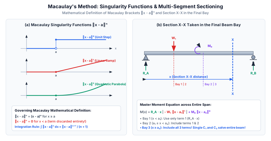
A single continuous differential equation is formulated for the entire beam by considering an arbitrary cross-section X−X located in the very last (rightmost) bay of the beam.
Every discontinuous load term is enclosed in special brackets ⟨x−a⟩.
By applying a specialized integration rule, the internal continuity conditions at all segment junctions are automatically satisfied by mathematical construction!
Consequently, only two constants of integration (C1 and C2) exist for the entire beam, regardless of whether there are 2, 5, or 10 point loads!
3. Mathematical Formulation of Macaulay's Bracket Notation
3.1 Definition of the Macaulay Singularity Bracket
The Macaulay bracket ⟨x−a⟩n (where a is the coordinate where the load originates) is defined mathematically as:
⟨x−a⟩n={(x−a)n0for x≥afor x<a
When evaluating slope or deflection at a point x to the left of the load (x<a), the quantity inside the bracket is negative; the entire bracket term is set to zero (discarded).
When x≥a, the bracket behaves exactly as an ordinary algebraic term (x−a)n.
3.2 The Sacred Macaulay Integration Rule
Unlike standard calculus where ∫(x−a)dx=2x2−ax, Macaulay brackets must always be integrated as a whole entity:
[!IMPORTANT]
Never expand the bracket term before integrating! Expanding ⟨x−a⟩2 as x2−2ax+a2 destroys the singularity property and invalidates the unification of constants C1 and C2.
4. Application to Standard Loading Elements
To write the master bending moment equation, section X−X is placed in the last segment at distance x from the left origin A:
EIdx2d2y=M(x)
Vertical divider lines (or dashes) are conventionally drawn to separate terms that become active in successive bays:
4.1 Concentrated Point Load W at x=a
Moment contribution at section x>a (hogging):
−W⟨x−a⟩1
First Integration (Slope contribution):
−2W⟨x−a⟩2
Second Integration (Deflection contribution):
−6W⟨x−a⟩3
4.2 Uniformly Distributed Load w Starting at x=a and Continuing to Free End
Moment contribution at section x>a:
−2w⟨x−a⟩2
First Integration:
−6w⟨x−a⟩3
Second Integration:
−24w⟨x−a⟩4
4.3 Concentrated Pure Moment / Couple M0 at x=a
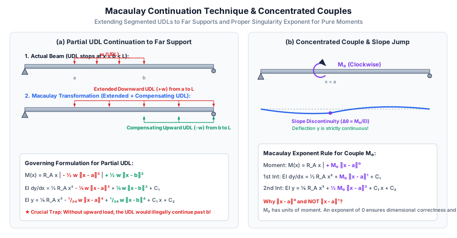
When a concentrated couple M0 acts at x=a (say, clockwise), it must be entered into the moment equation with an exponent of zero:
+M0⟨x−a⟩0
Why exponent 0 is mandatory:
Dimensional Homogeneity: M0 is already a moment (N⋅mm). Multiplying by a distance (x−a) would yield N⋅mm2, which is dimensionally incorrect.
Physical Kinematics:
First integration yields:
∫M0⟨x−a⟩0dx=M0⟨x−a⟩1
which creates a sudden finite jump (kink) in the slope θ of magnitude Δθ=M0/EI across x=a.
Second integration yields:
∫M0⟨x−a⟩1dx=2M0⟨x−a⟩2
which evaluates to zero at x=a, guaranteeing that the vertical deflection y remains perfectly continuous!
5. The Partial UDL Continuation Technique
5.1 The Mathematical Dilemma of Segmented UDLs
Macaulay brackets possess an automatic "turn-on" mechanism at x=a, but they have no built-in "turn-off" mechanism:
If a UDL of intensity w starts at x=a and terminates at x=b (b<L), writing −2w⟨x−a⟩2 applies the load across the entire remainder of the beam from a all the way to L!
5.2 The Continuation & Compensation Principle
To maintain a single unified equation:
Extend the downward UDL of intensity w from its cutoff point x=b continuously to the far right end L.
Compensate simultaneously by applying an equal, opposite upward UDL of intensity −w starting at x=b and extending to the far right end L.
The net physical load between b and L is (+w)+(−w)=0, exactly restoring the original unloaded state!
The resulting bending moment expression is:
M(x)=RAx−2w⟨x−a⟩2+2w⟨x−b⟩2
For x<a: Neither bracket is active; M(x)=RAx.
For a≤x<b: Only the first bracket is active; M(x)=RAx−2w(x−a)2.
For x≥b: Both brackets are active; the second bracket cancels the extended portion of the first bracket!
6. Determination of Integration Constants C1 and C2
For a simply supported beam of span L supported at x=0 (A) and x=L (B):
At Support A (x=0):
The deflection is zero: y(0)=0.
Since x=0 lies in the first segment (before any internal loads), all Macaulay brackets ⟨0−a⟩ are negative and drop out:
EI(0)=RA6(0)3+C1(0)+C2⟹C2=0
[!TIP]
For any beam whose origin x=0 is a simple pin/roller support or fixed support, C2 is always identically zero.
At Support B (x=L):
The deflection is zero: y(L)=0.
Because x=L lies at the extreme right end, every single Macaulay bracket term is active (L>a, L>b):
0=RA6L3−∑6Wi(L−ai)3−∑24wj(L−aj)4+C1L
Solving this linear algebraic equation directly gives the unique value of C1.
7. SVG Technical Diagrams & Visual Explanations
7.1 Singularity Bracket Functions & Section X-X in Final Bay
The diagram below illustrates the mathematical functions ⟨x−a⟩n for step, ramp, and quadratic profiles, along with the sectioning protocol across multi-bay beams:
The diagram below depicts the extension and compensatory loading for partial UDLs and the slope-step behavior of concentrated moments:
8. Step-by-Step Solved Numerical Examples
Problem 1: Simply Supported Beam with Eccentric Point Load (GATE CE Pattern)
Statement:
A simply supported beam of span L=6.0 m carries a single concentrated load W=60 kN at a distance a=2.0 m from the left support A (so b=4.0 m to right support B). Given flexural rigidity EI=2.0×10¹³ N⋅mm2:
Formulate the unified Macaulay differential equation for the entire beam.
Calculate the integration constants C1 and C2.
Determine the slope at both supports (θA and θB).
Compute the vertical deflection directly under the load (yload).
Determine the location (xmax) and magnitude (δmax) of the absolute maximum deflection.
Solution:
Step 1: Support Reactions
ΣMB=0⟹RA×6.0−60×4.0=0⟹RA=6240=40 kN=40000 NΣFy=0⟹RB=60−40=20 kN=20000 N
At x=0, y=0: The bracket term drops out:
0=0+0+C2⟹C2=0
At x=L=6000 mm, y=0: The bracket is active:
0=320000(6000)3+C1(6000)−10000(6000−2000)3(6000)3=2.16×10¹¹⟹320000×2.16×1011=1.44×10¹⁵ N⋅mm3(4000)3=6.4×10¹⁰⟹10000×6.4×1010=6.4×10¹⁴ N⋅mm30=1.44×10¹⁵−6.4×10¹⁴+6000C16000C1=−8.0×10¹⁴⟹C1=−1.33333×10¹¹ N⋅mm2
Step 4: Slopes at Supports
At support A (x=0): Bracket drops out:
θA=dxdy0=EIC1=2.0×10¹³−1.33333×1011=−0.006667 rad=−0.382∘
At support B (x=6000 mm):
EIθB=20000(6000)2−1.33333×10¹¹−30000(4000)2EIθB=7.20×10¹¹−1.33333×10¹¹−4.80×1011=+1.06667×10¹¹θB=2.0×10131.06667×1011=+0.005333 rad=+0.306∘
Trial in Left Segment (0≤x≤2000 mm, where the Macaulay bracket is inactive):EIdxdy=20000x2+C1=0⟹20000x2=1.33333×10¹¹⟹x2=6.66667×106 mm2xtrial=6.66667×106=2581.99 mm>2000 mm
Since 2581.99 mm>2000 mm, the point of zero slope lies in the longer right segment (2000 mm<x≤6000 mm).
Exact Solution in Right Segment (x>2000 mm, Macaulay bracket active):
Setting dxdy=0 in Eq. 1 for x>2000 mm:
20000x2−1.33333×10¹¹−30000(x−2000)2=020000x2−1.33333×10¹¹−30000(x2−4000x+4×10⁶)=0−10000x2+1.2×10⁸x−2.53333×1011=0⟹x2−12000x+25333333.3=0
Solving the quadratic equation (selecting the root within 2000<x<6000 mm):
xmax=212000−144×106−101.3333×106=212000−6531.97=2734.01 mm from support A(Standard closed-form verification measuring from the farther support B, where b=4000 mm>a=2000 mm: xmax=L−3L2−a2=6000−336−4×106=6000−3265.99=2734.01 mm).
Maximum Downward Deflection:
Substituting x=2734.01 mm into Eq. 2 gives:
ymax=−11.476 mm
Problem 2: Beam with Symmetrical Partial UDL (UPSC ESE Pattern)
Statement:
A simply supported beam of span L=8.0 m carries a uniformly distributed load w=24 kN/m spanning over its central 4.0 m length (from x=2.0 m to x=6.0 m). Flexural rigidity EI=4.0×10¹³ N⋅mm2.
Apply the continuation trick to formulate the Macaulay bending moment equation.
Solve for integration constant C1.
Compute the maximum deflection at midspan (x=4.0 m).
Solution:
Step 1: Support Reactions
By symmetry, the load of 24 kN/m×4.0 m=96 kN is shared equally:
RA=RB=296=48 kN=48000 N
Step 2: Formulate Macaulay Equations with Continuation
Extend the downward UDL from x=6000 mm to 8000 mm, and compensate with an upward UDL starting at x=6000 mm:
At x=8000 mm, y=0 (all brackets active):
0=8000(8000)3+C1(8000)−(8000−2000)4+(8000−6000)48000×(5.12×1011)=4.096×10¹⁵−(6000)4=−1.296×10¹⁵+(2000)4=+1.60×1013=+0.016×10¹⁵Net=4.096×10¹⁵−1.296×10¹⁵+0.016×1015=2.816×10158000C1=−2.816×10¹⁵⟹C1=−3.520×10¹¹ N⋅mm2
Step 4: Midspan Deflection (x=4000 mm)
At midspan x=4000 mm, the first bracket is active (4000−2000=2000), while the second bracket is inactive (4000<6000):
Problem 3: Beam with Concentrated Couple M0 (State AE Pattern)
Statement:
A simply supported beam of span L=6.0 m carries a single clockwise concentrated couple M0=36 kN⋅m (3.6×10⁷ N⋅mm) at distance a=2.0 m from left support A. Given EI=3.0×10¹³ N⋅mm2, determine:
Support reactions RA and RB.
The Macaulay slope and deflection equations.
Slopes at both supports (θA and θB).
The deflection under the applied couple.
Solution:
Step 1: Reactions
Clockwise couple M0 requires an anti-clockwise reaction couple:
ΣMA=0⟹M0−RB⋅L=0⟹RB=LM0=6.036=+6.0 kN=+6000 N (Upward)ΣFy=0⟹RA=−RB=−6.0 kN=−6000 N (Downward!)
At x=6000 mm, y=0:
0=−1000(6000)3+C1(6000)+1.8×10⁷(6000−2000)2−1000×2.16×1011=−2.16×10141.8×107×(1.6×107)=+2.88×10140=+0.72×10¹⁴+6000C1⟹6000C1=−7.2×10¹³C1=−1.200×10¹⁰ N⋅mm2
Step 4: Slopes and Deflection
Slope at Support A (x=0):
θA=EIC1=3.0×10¹³−1.200×1010=−0.000400 rad=−0.0229∘
Slope at Support B (x=6000 mm):
EIθB=−3000(6000)2−1.20×10¹⁰+3.6×10⁷(4000)EIθB=−1.08×10¹¹−0.12×10¹¹+1.44×1011=+0.24×10¹¹θB=3.0×10132.40×1010=+0.000800 rad=+0.0458∘
Deflection at Couple Location (x=2000 mm):
EIy(2000)=−1000(2000)3+(−1.20×10¹⁰)(2000)+0EIy(2000)=−8.0×10⁹−2.4×1010=−3.20×10¹⁰ N⋅mm3ycouple=3.0×10¹³−3.20×1010=−1.067 mm(Downward)
9. Comparative Analysis & Summary Matrix
Method
Number of Unknown Constants
Handling of Interior Point Loads
Handling of Partial UDLs
Best Exam Suitability
Direct Double Integration
2n (n=number of segments)
Must set up n separate ODEs with interface matching
Extremely cumbersome algebra
Single continuous load across whole span
Macaulay's Method
Always Exactly 2 (C1,C2)
Single equation with ⟨x−a⟩1 brackets
Simple continuation with compensating upward UDL
Multiple point loads, couples, and partial UDLs
Moment-Area Method (Mohr)
0 (Geometric integration)
Requires drawing M/EI diagrams and calculating areas/centroids
Moderate complexity for multi-segment centroids
Non-prismatic beams, cantilevers, symmetric spans
Conjugate Beam Method
0 (Fictitious beam analysis)
Deflection equals bending moment of fictitious beam
Requires solving fictitious beam shear and moments
Non-uniform EI and fixed/continuous supports
10. Key Takeaways & Exam-Oriented Highlights
Section X-X Placement Rule: Always place the cutting section in the very last (rightmost) bay so that every load on the span appears in the master equation.
Integral Power Rule:
Point load: ∫⟨x−a⟩1dx=2⟨x−a⟩2⟹∬=6⟨x−a⟩3.
UDL: ∫⟨x−a⟩2dx=3⟨x−a⟩3⟹∬=12⟨x−a⟩4.
Couple: ∫⟨x−a⟩0dx=⟨x−a⟩1⟹∬=2⟨x−a⟩2.
Partial UDL Rule: If a UDL does not go to the right end, extend it and add a compensating upward load.
Max Deflection Location for Eccentric Point Load:
The maximum deflection never occurs under the load itself (unless centered). It always shifts toward the center inside the longer segment at:
xmax=3L2−b2(measured from support nearest the load)δmax=93EILWb(L2−b2)3/2
11. Common Traps, Pitfalls & Counter-Intuitive Exam Scenarios
Trap 1: Expanding Macaulay Brackets: Misconception: Writing ⟨x−2⟩2=x2−4x+4. Correction: Never expand! Integrating expanded polynomials violates the singularity condition when x<2.
Trap 2: Using Exponent 1 for Pure Couples: Misconception: Writing M0⟨x−a⟩1. Correction: This has units of N⋅mm2, which corrupts dimensions and prevents the slope jump. The exponent must be 0 (M0⟨x−a⟩0).
Trap 3: Forgetting Upward Compensating UDL: Misconception: Entering only −2w⟨x−a⟩2 when UDL terminates at x=b. Correction: This erroneously continues the UDL across the whole beam. You must add +2w⟨x−b⟩2.
Trap 4: Discarding Positive Bracket Values: Misconception: Forgetting that when x≥a, the bracket is strictly active and evaluated as (x−a).
12. Standard Code Provisions & Objective Practice Problems
Reference Code Clauses
IS 456:2000 Cl. 23.2 & IS 800:2007 Table 6:
Structural safety standards mandate that calculated elastic deflections using Macaulay's method must be compared against span-to-depth ratios and absolute deflection limits (Span/250 for total load, Span/300 for live load on steel beams).
Objective Practice Problems
Problem 1 (GATE CE)
In Macaulay's method, the bending moment due to a concentrated couple M acting clockwise at distance a from the origin is written as:
(A) M⟨x−a⟩1
(B) M⟨x−a⟩0
(C) 2M⟨x−a⟩2
(D) M(x−a)
Answer:(B) Solution:
A concentrated couple has units of moment and must be entered as M⟨x−a⟩0 so that upon integration it yields slope step M⟨x−a⟩1 and continuous deflection 2M⟨x−a⟩2.
Problem 2 (UPSC ESE)
A simply supported beam of span L carries a concentrated load W at distance a from the left support (a<L/2). The maximum deflection of the beam occurs:
(A) Exactly at midspan (x=L/2)
(B) Directly under the concentrated load (x=a)
(C) Between the load and the midspan
(D) Outside the span
Answer:(C) Solution:
For an eccentric load, the point of zero slope (and hence maximum deflection) always lies between the concentrated load and the midspan inside the longer segment at x=(L2−b2)/3 from the closer support.
Problem 3 (SSC JE / RRB JE)
When applying Macaulay's method to a beam carrying a partial UDL that does not extend to the right support, the procedure required is:
(A) Ignore the load after the cutoff point
(B) Extend the load to the right support and add an equal upward UDL from the cutoff point
(C) Integrate backwards from the right support
(D) Use direct double integration instead
Answer:(B) Solution:
Macaulay brackets do not switch off automatically; the load must be extended to the right end and balanced by a fictitious upward compensating UDL from the cutoff point to the right end.
Problem 4 (GATE CE)
A simply supported beam of span L=6 m carries an eccentric load W=30 kN at a=2 m from left support A (b=4 m). The distance of the point of maximum deflection from support A is:
(A) 2.00 m
(B) 2.58 m
(C) 2.73 m
(D) 3.00 m
Answer:(C) Solution:
The longer segment is on the right (b=4 m). Measuring from support B, the maximum deflection is at distance xB=(L2−a2)/3=(36−4)/3=10.67=3.266 m.
Therefore, the distance from support A is xA=6.000−3.266=2.734 m≈2.73 m.
Problem 5 (State AE / ESE)
In Macaulay's method, what is the value of the integration constant C2 for a simply supported beam with origin at the left pinned support?
(A) WL2/16
(B) wL3/24
(C) 0
(D) Depends on the magnitude of the loads
Answer:(C) Solution:
At x=0, y=0. Since all loads lie at x>0, all Macaulay brackets are negative and evaluate to zero, leaving 0=0+0+C2⟹C2=0.