Load, Shear Force, and Bending Moment Differential Relations
In this chapter (4 topics)
On this page
- 1. Topic Metadata
- 2. Physical Mechanics & Theoretical Foundation
- Physical Meaning of the Differential Relationships:
- 3. Mathematical Derivations & Governing Equations
- 3.1 Sign Convention
- 3.2 Vertical Equilibrium of Element dx
- 3.3 Rotational Equilibrium of Element dx
- 3.4 Polynomial Degree Progression Hierarchy
- 3.5 Critical Stationary Points and Singularities
- 4. Engineering Assumptions & Validity Limits
- 5. SVG Technical Illustrations & Diagrammatic Analysis
- Figure 1: Infinitesimal Beam Element Equilibrium
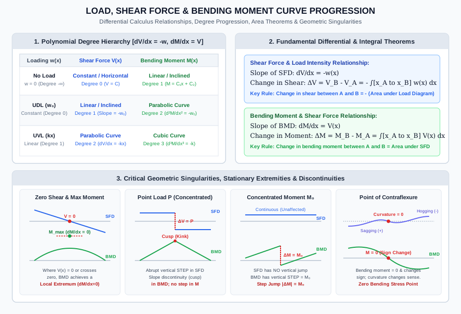
- Figure 2: Load, Shear, and Moment Curve Progression & Critical Singularities
- 6. Solved Numerical Examples (Python-Verified)
- Example 1: Simply Supported Beam under Linearly Varying Load (UVL) — Peak Moment by Differential Calculus
- Example 2: Beam Subjected to Concentrated Couple, Point Load, and UDL — Piecewise Integration & Discontinuity Analysis
- Example 3: Cantilever Beam under Symmetric Parabolic Loading — Boundary Value Problem
- 7. Engineering Applications & Real-World Case Studies
- 8. Comparative Analysis & Summary Matrix
- 9. Key Takeaways & Exam-Oriented Mnemonics
- 10. Common Pitfalls, Traps & Misconceptions
- 11. Standard Specifications & Code Provisions
- 12. Comprehensive Formula Box & Practice Problems
- Governing Formula Summary
- Practice Problems
1. Topic Metadata
| Field | Detail |
|---|---|
| Topic Identifier | SOM-03-02 |
| Subject | Strength of Materials / Solid Mechanics |
| Chapter | Shear Force and Bending Moment Diagrams (SFD & BMD) |
| Difficulty Level | Intermediate to Advanced |
| Target Examinations | GATE CE, UPSC ESE, SSC JE, State AE/JE, RRB JE |
| Primary Prerequisites | Static Equilibrium (), Infinitesimal Differential Elements, Free-Body Diagrams |
| Governing Relations | , , |
| Authoritative Code References | IS 456:2000, IS 800:2007, IRC:112-2020 |
2. Physical Mechanics & Theoretical Foundation
In beam mechanics, the internal resultant actions—specifically the shear force and bending moment —are not isolated quantities. They represent continuous spatial distributions that equilibrate the externally applied distributed and concentrated forces.
The relationship between the external distributed transverse load intensity , the internal transverse shear force , and the internal bending moment is governed rigorously by the equilibrium of an infinitesimal beam segment of length .
Physical Meaning of the Differential Relationships:
-
Load Intensity as the Slope of the Shear Force Diagram: The transverse load intensity (expressed in or ) represents the rate of change of the shear force along the beam axis. A downward distributed load continuously decreases the internal shear force as one progresses from left to right:
Consequently, the negative slope of the Shear Force Diagram (SFD) at any coordinate equals the distributed load intensity at that point.
-
Shear Force as the Slope of the Bending Moment Diagram: The internal shear force (expressed in or ) represents the spatial gradient (rate of change) of the bending moment along the beam axis:
Consequently, the slope of the Bending Moment Diagram (BMD) at any coordinate is equal to the magnitude and sign of the shear force at that section.
-
Curvature of the Bending Moment Diagram: Combining both relations reveals that the second spatial derivative of the bending moment corresponds directly to the negative of the distributed load intensity:
This implies that wherever a beam carries a downward distributed load (), , which signifies that the bending moment curve is strictly concave downward (negative curvature).
3. Mathematical Derivations & Governing Equations
Consider an infinitesimal beam element of length extracted from an arbitrarily loaded beam between section and section .
                 w(x) [Downward Distributed Load]
             ↓↓↓↓↓↓↓↓↓↓↓↓↓↓↓↓↓↓↓↓
          ┌────────────────────────┐
          │                        │
  V(x)    │                        │    V(x) + dV
   ↑      │       Beam Element     │       ↓
          │                        │
  M(x) ↷  │       Length dx        │    ↷ M(x) + dM
          └────────────────────────┘
          |←────────── dx ────────→|
3.1 Sign Convention
We establish the universal civil engineering sign convention:
- Shear Force (): Positive if it produces a clockwise shearing couple on the segment (i.e., upward on the left face, downward on the right face).
- Bending Moment (): Positive if it produces sagging curvature (tensile strain at the bottom fibers, compressive strain at the top fibers; i.e., clockwise on the left face, counter-clockwise on the right face).
- Distributed Load (): Positive downwards ().
3.2 Vertical Equilibrium of Element
Summing all vertical forces on the element (, upward positive):
Canceling :
Dividing through by the differential length :
Integrating both sides between two sections () and ():
First Integral Principle: The change in shear force between any two sections along a beam equals the negative of the total distributed load (area under the load curve) acting between those two sections.
3.3 Rotational Equilibrium of Element
Summing moments about the center of the right face at section (, counter-clockwise positive):
Simplifying:
The third term contains , which is a second-order infinitesimal quantity. In the limit as , vanishes compared to the first-order differential terms:
Integrating both sides between section and section :
Second Integral Principle: The change in bending moment between any two sections along a beam equals the algebraic area under the shear force diagram between those two sections.
3.4 Polynomial Degree Progression Hierarchy
Because differentiation reduces polynomial order by 1, and integration increases polynomial order by 1, the curve degree progresses sequentially across load, shear, and moment:
| Loading Condition | Load Degree | Shear Force Curve | Shear Degree | Bending Moment Curve | Moment Degree |
|---|---|---|---|---|---|
| No Distributed Load () | Horizontal line () | Inclined straight line () | |||
| Uniformly Distributed Load (UDL) () | Inclined straight line () | Parabolic curve () | |||
| Uniformly Varying Load (UVL) () | 2nd-degree parabola () | 3rd-degree cubic parabola () | |||
| Parabolic Load () | 3rd-degree cubic parabola () | 4th-degree quartic curve () |
3.5 Critical Stationary Points and Singularities
1. Maximum and Minimum Bending Moment
From standard differential calculus, an extremum of a differentiable function occurs where its first derivative vanishes:
- If the shear force passes continuously through zero from positive to negative (), the bending moment attains a local maximum.
- If the shear force passes through zero from negative to positive, the bending moment attains a local minimum.
- If a concentrated point load causes the shear force to abruptly cross the zero baseline with a step discontinuity, the maximum bending moment occurs at that exact point load location (forming a sharp cusp or kink in the BMD).
2. Point of Contraflexure (Point of Inflection)
A point of contraflexure (or point of inflection) is defined as a point along the beam where the internal bending moment changes algebraic sign ( with sign reversal).
- Physically, the beam cross-section transitions from sagging curvature (concave up) to hogging curvature (concave down).
- At this section, the normal bending stresses throughout the beam cross-section are identically zero ().
3. Step Discontinuities under Concentrated Actions
- Concentrated Transverse Point Load (): A concentrated load produces an instantaneous vertical step jump of magnitude in the SFD. The bending moment diagram remains continuous but experiences an abrupt change in slope (), producing a sharp cusp.
- Concentrated Applied Moment / Couple (): A concentrated moment causes an instantaneous vertical step jump of magnitude in the BMD without causing any step change in the SFD.
4. Engineering Assumptions & Validity Limits
- Euler-Bernoulli Beam Kinematics: The beam is straight, prismatic (or slightly tapering), and has a longitudinal plane of symmetry in which all applied loads act.
- Small Deflections & Rotations: The deflections and rotations are sufficiently small such that the geometry of the beam does not change appreciably under load ().
- Linear Elastic & Isotropic Material: Stress is directly proportional to strain (). The cross-sectional dimensions remain constant along the infinitesimal length .
- Neglect of Shear Deformation on Equilibrium: The shear forces are accounted for in cross-sectional equilibrium, but higher-order Timoshenko shear distortion effects on beam curvature are neglected.
- Static Transverse Loading: Dynamic inertia effects () are zero; all forces are applied statically.
5. SVG Technical Illustrations & Diagrammatic Analysis
Figure 1: Infinitesimal Beam Element Equilibrium
The following diagram illustrates the complete free-body equilibrium of a differential slice subject to a transverse distributed load , showing internal shearing forces and bending couples acting on adjacent transverse faces.
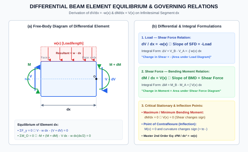
Figure 2: Load, Shear, and Moment Curve Progression & Critical Singularities
The diagram below presents the polynomial degree progression hierarchy, the fundamental area theorems, and the four canonical geometric conditions: zero shear extremum, point load discontinuity, concentrated couple step jump, and point of contraflexure.
6. Solved Numerical Examples (Python-Verified)
Example 1: Simply Supported Beam under Linearly Varying Load (UVL) — Peak Moment by Differential Calculus
Problem Statement: A simply supported beam of span carries a uniformly varying load that increases linearly from zero intensity at support () to a maximum intensity of at support (). Using differential equations:
- Determine the support reactions and .
- Formulate the general expressions for shear force and bending moment .
- Locate the coordinate of maximum bending moment and calculate its exact magnitude.
- Verify the curvature condition at the stationary point.
          w = 0 at A                          w_0 = 18 kN/m at B
              /|                              ▲
             / |                              │
            /  |   Uniformly Varying Load     │
           /   |   w(x) = (w_0 / L) * x       │
          /    |                              │
       ▲ ──────┴──────────────────────────────▲
       A (x = 0)                           B (x = 6 m)
       |<────────────── L = 6 m ─────────────>|
Solution & Step-by-Step Mathematical Derivation:
Step 1: Calculate Global Support Reactions: Total downward load on the beam:
The centroid of the triangular load is located at a distance of from support . Taking moments about support (, clockwise positive):
From vertical equilibrium ():
Step 2: Formulate Differential Equations and Boundary Conditions: The load intensity at any distance from is:
Applying the first governing differential relation:
Integrating with respect to :
Boundary condition at (just to the right of support reaction ):
Thus, the shear force equation is:
(Note: At , , perfectly verified!)
Applying the second governing differential relation:
Integrating with respect to :
Boundary condition at the simple pin support ():
Thus, the bending moment equation is:
(Check at : , perfectly verified!)
Step 3: Determine Stationary Extremum of Bending Moment: Setting the first derivative of (which is ) to zero:
In algebraic form:
Substitute into the bending moment equation:
Standard closed-form formula verification:
Step 4: Second Derivative Curvature Verification:
Because the second derivative is strictly negative, the stationary point is guaranteed to be a strict local maximum.
Example 2: Beam Subjected to Concentrated Couple, Point Load, and UDL — Piecewise Integration & Discontinuity Analysis
Problem Statement: A beam of span is simply supported at () and (). It is subjected to:
- A concentrated clockwise couple at .
- A concentrated downward point load at .
- A uniformly distributed load extending over the right half from to .
Determine:
- Support reactions and .
- Piecewise functions for and across all zones.
- The magnitudes of the step discontinuities in SFD and BMD.
- The location and magnitude of the absolute maximum bending moment.
- Verify the results using the Area Theorems.
Solution:
Step 1: Global Reactions: Taking moments about (, clockwise positive):
From vertical equilibrium ():
Step 2: Piecewise Governing Functions:
-
Zone 1: (Unloaded segment):
At : . At : .
-
Singularity at (Clockwise Couple ): The shear force is completely continuous across :
In the sagging-positive sign convention, an external clockwise couple to the left of the cut adds positive rotational work:
-
Zone 2: (Unloaded segment):
At : .
-
Singularity at (Point Load ): The downward point load introduces an instantaneous downward vertical drop in the SFD:
The bending moment is continuous across :
Notice that the slope abruptly changes from to , forming a sharp cusp.
-
Zone 3: (UDL ):
At : .
At :
Boundary condition at the right hinge support is satisfied identically!
Step 3: Identification of Absolute Maximum Bending Moment: Because the shear force transitions from positive () to negative () by crossing zero at , the absolute maximum bending moment occurs at :
Step 4: Verification via Area Theorems:
- Change in Moment between and :
- Jump at : .
- Change in Moment between and :
- Change in Moment between and :
Example 3: Cantilever Beam under Symmetric Parabolic Loading — Boundary Value Problem
Problem Statement: A cantilever beam of length is rigidly clamped at support () and has a completely free end at (). It is subjected to a continuous parabolic distributed load given by:
where . Using the differential equations of equilibrium:
- Determine the shear force function and find the support reaction at the fixed support.
- Determine the bending moment function and evaluate the fixed-end moment .
- Sketch the qualitative nature of and .
Solution:
Step 1: Integration for Shear Force : The differential relation states:
Integrating with respect to :
Boundary condition at the free end (): At a free end without concentrated end loads, the shear force must vanish:
Substituting :
Support Reaction at fixed base ():
Step 2: Integration for Bending Moment : The differential relation states:
Integrating with respect to :
Boundary condition at the free end (): At a free end without concentrated end couples, the bending moment must vanish:
Substituting into :
Fixed-End Bending Moment at ():
The negative sign confirms that the cantilever fixed base experiences a hogging bending moment of magnitude (top fibers in tension).
7. Engineering Applications & Real-World Case Studies
- Structural Steel Framing & Shear Wall Interconnections (IS 800:2007): In multi-story steel frames, beam-to-column connections are designed as either "shear-only (simple)" or "moment-resisting (rigid)". The equation dictates that at connection interfaces, high shear values produce rapid changes in moment. Engineers locate splices where is minimal (near points of contraflexure) to drastically reduce the required flange splice plate thickness.
- Reinforced Concrete Flexural Design & Reinforcement Curtailment (IS 456:2000 Cl. 26.2.3): Tensile steel reinforcement is required to resist flexural tension governed by . Rather than extending 100% of the longitudinal rebars across the entire span, engineers curtail rebars at locations where the moment capacity envelope comfortably exceeds the actual curve. The differential slope dictates the bond stress that must be developed between concrete and steel to transfer flexural tension along the rebar.
- Bridge Girder Web Panel Design & Shear Buckling (IRC:24-2010): In plate girders under vehicular traffic, transverse web stiffeners are spaced closer together near the supports where is maximal, and spaced farther apart toward midspan where . Conversely, the girder flange plates reach maximum thickness at midspan where .
- Highway Pavement & Retaining Wall Base Slabs: In inverted cantilevers (such as base slabs of cantilever retaining walls), upward soil reaction pressures are modeled as trapezoidal loads. Integrating gives the shear demand for diagonal tension shear checks, and the second integral gives the flexural steel demand.
8. Comparative Analysis & Summary Matrix
| Characteristic | Shear Force | Bending Moment |
|---|---|---|
| Physical Definition | Net transverse internal force balancing external loads | Net internal rotational couple balancing external moments |
| Differential Relationship | ||
| Geometric Slope Meaning | Slope of SFD = Negative of load intensity () | Slope of BMD = Shear force () |
| Area Theorem | (Negative area under load diagram) | (Algebraic area under SFD) |
| Effect of Point Load | Vertical step jump equal to load magnitude () | Continuous curve with a sharp slope cusp () |
| Effect of Concentrated Couple | Unaffected; completely continuous () | Vertical step jump equal to couple magnitude () |
| Stationary Extremum Condition | (occurs where load is zero) | (occurs where shear is zero or changes sign) |
| Point of Zero Value () | Point where slope of BMD is horizontal | Point of Contraflexure (if sign changes; zero bending stress) |
9. Key Takeaways & Exam-Oriented Mnemonics
- Mnemonic for Curve Degrees: is :
- No load: is constant (Degree 0) is linear (Degree 1).
- UDL: (Degree 0) is linear (Degree 1) is 2nd-degree parabolic (Degree 2).
- UVL: is linear (Degree 1) is 2nd-degree parabolic (Degree 2) is 3rd-degree cubic (Degree 3).
- The "Zero Shear = Peak Moment" Golden Rule:
- Wherever the shear force crosses zero, the bending moment is at a local maximum or minimum.
- GATE/ESE Trap: In beams with point loads, shear may cross zero with an instantaneous step change rather than a smooth zero slope. The peak moment still occurs at that section!
- Concentrated Action Jump Rules:
- Point Load Jump in SFD only.
- Concentrated Couple Jump in BMD only.
10. Common Pitfalls, Traps & Misconceptions
[!WARNING] Pitfall 1: Confusing the Direction of Jump for Concentrated Couples A common exam trap involves determining whether a clockwise couple causes an upward or downward jump in the BMD. Under the standard sagging-positive convention ( on the left is positive), passing a clockwise couple from left to right causes an upward step jump of . Always verify by computing the moment from both the left and right sides of the section!
[!CAUTION] Pitfall 2: Forgetting that Maximum Moment Can Occur at a Point of Non-Differentiability Students often assume that is the only way to locate maximum moment. If a concentrated load is present, does not exist at that point because the left-hand derivative () differs from the right-hand derivative (). If is positive and is negative, the maximum moment occurs at the cusp!
[!NOTE] Pitfall 3: Assuming Point of Zero Moment is Always a Point of Contraflexure A simply supported end has , but it is not a point of contraflexure because the bending moment does not cross the baseline to reverse sign. An internal point of contraflexure requires curvature reversal (transition between sagging and hogging).
11. Standard Specifications & Code Provisions
| Standard | Clause / Section | Engineering Requirement |
|---|---|---|
| IS 456:2000 | Cl. 26.2.3.1 | Flexural reinforcement curtailment must account for the shift in tension force due to diagonal cracking (the "-spread" or tension shift rule: bars must extend by effective depth beyond the theoretical cut-off point determined from ). |
| IS 456:2000 | Cl. 22.5.1 | Critical section for shear force in beams with compressive reactions: design shear force may be taken at a distance from the support face, reflecting load dispersion into the support. |
| IS 800:2007 | Cl. 8.2.1 | Design bending strength of steel I-sections under high shear: when factored shear force , plastic moment capacity must be reduced to to account for shear-moment interaction ( yield envelope). |
| IRC:112-2020 | Cl. 10.3.2 | Shear resistance without shear reinforcement in bridge decks based on calculated from differential area theorems under IRC Class A and Class 70R wheel loads. |
12. Comprehensive Formula Box & Practice Problems
Governing Formula Summary
Practice Problems
-
(GATE CE Pattern) A simply supported beam of span carries a uniformly distributed load of on its left half (from to ). Find the exact distance from the left support where the bending moment is maximum, and determine .
- Answer: . Since and load is , shear force reaches zero at . .
-
(UPSC ESE Pattern) A cantilever beam of length carries a distributed load of intensity measuring from the free end ( at free end, at fixed base). Find the ratio of the bending moment at midspan to the bending moment at the fixed base.
- Answer: At any distance from free end, . . At midspan (): . At fixed base (): . Ratio .
-
(State AE Pattern) A beam carries an external clockwise concentrated moment at midspan. Which of the following statements is FALSE?
- (A) The shear force is constant across the entire span.
- (B) The bending moment diagram has a vertical step jump of magnitude at midspan.
- (C) The shear force diagram has a vertical step jump of magnitude at midspan.
- (D) The reactions at the two end supports are equal and opposite.
- Answer: (C) is FALSE. A concentrated moment produces zero discontinuity in the shear force diagram ().