Concept of Stress, Strain & Constitutive Relations
In this chapter (6 topics)
On this page
- 1. Executive Summary & Core Definitions
- 1.1 Definition of Stress (σ, τ)
- 1.2 SI Units and Dimensional Analysis
- 1.3 Definition of Strain (ε, γ)
- 2. Fundamental Physical Principles & Theory
- 2.1 The Concept of Internal Resistance: Why Stress ≠ Pressure
- 2.2 Saint-Venant's Principle
- 3. Governing Mathematical Formulations & Derivations
- 3.1 The Cauchy Stress Tensor (3D State of Stress)
- 3.2 Proof of Complementary Shear Stress Equality
- 3.3 Mathematical Formulation of Shear Strain (γ)
- 3.4 Engineering Stress-Strain vs True (Natural) Stress-Strain
- 4. Fundamental Assumptions & Limitations of Elastic Mechanics
- 5. Indian Standard (IS) Code Relevance
- 5.1 IS 456:2000 (Plain and Reinforced Concrete)
- 5.2 IS 800:2007 (General Construction in Steel)
- 6. Comparative Analysis
- 7. Step-by-Step Solved Numerical Examples
- Example 1.1: Prismatic Tensile Bar with Independent Recalculation (SSC JE / State AE Level)
- Example 1.2: True Stress vs Engineering Stress at High Strain (GATE CE Level)
- Example 1.3: Shear Stress and Angular Distortion in a Rubber Bearing Pad (UPSC ESE Level)
- 8. Common Pitfalls & Competitive Exam Traps
- 9. Quick Revision Formula Box
- 10. References & Source Literature
1. Executive Summary & Core Definitions
In structural and civil engineering, understanding how deformable bodies respond to external forces is fundamental to ensuring safety, serviceability, and economy.
                          EXTERNAL FORCES (Loads)
                                     │
                                     ▼
                        DEFORMATION OF SOLID BODY
                                     │
                                     ▼
                   INTERNAL RESISTING FORCES DEVELOPED
                                     │
                  ┌──────────────────┴──────────────────┐
                  ▼                                     ▼
        INTENSITY PER UNIT AREA                DEFORMATION PER UNIT LENGTH
          [ STRESS : σ, τ ]                       [ STRAIN : ε, γ ]
1.1 Definition of Stress ()
When an external force system acts on a deformable body, the internal atoms and grains of the material exert resisting forces to counteract the applied loads and preserve structural equilibrium.
Scientific Definition: Stress is the intensity of internal resisting force developed per unit area of a body across an internal plane passing through a point.
Mathematically, considering an infinitesimal internal plane of area subjected to an internal resisting force vector :
The internal force vector is resolved into two mutually perpendicular components:
- Normal Force (): Acting perpendicular (orthogonal) to the plane. The resulting intensity is the Normal Stress ():
- Tensile Stress (): Tends to pull, stretch, or elongate the fibers away from the cross-section.
- Compressive Stress (): Tends to push, squash, or shorten the fibers toward the cross-section.
- Tangential Force (): Acting parallel (tangent) to the plane. The resulting intensity is the Shear Stress ():
1.2 SI Units and Dimensional Analysis
- SI Unit of Stress: Pascal ().
- Civil Engineering Common Multiples:
- Megapascal:
- Gigapascal:
- Kilonewton per square meter:
- Dimensional Formula:
1.3 Definition of Strain ()
When a solid material experiences stress, it undergoes physical deformation and geometric distortion.
Scientific Definition: Strain is a dimensionless geometric measure of deformation representing the relative displacement between particles within a material body.
- Normal Strain (): The change in linear dimension per unit original dimension:
- Tensile Strain (): Increase in length along the direction of loading.
- Compressive Strain (): Decrease in length along the direction of loading.
- Shear Strain (): The angular distortion between two mutually perpendicular line segments in an undeformed element, measured in radians: where is the final angle between the two lines in the deformed state.
- Volumetric Strain (): The fractional change in volume of a body: For small deformations in Cartesian space:
2. Fundamental Physical Principles & Theory
2.1 The Concept of Internal Resistance: Why Stress Pressure
Although both stress and pressure share the same SI units ( or ), they represent physically distinct concepts in mechanics:
| Parameter | Stress () | Pressure () |
|---|---|---|
| Physical Nature | Internal reaction developed inside the material to resist external forces. | External contact force applied onto the surface of a body by an external agent (fluid, gas, contact). |
| Directionality | Can be normal (tensile/compressive) or tangential (shear). | Strictly normal and always compressive in fluids (). Fluids cannot sustain static tension. |
| Mathematical Nature | Second-order tensor (9 components in 3D space). | Scalar quantity (isotropic in static fluids per Pascal's Law). |
| Measurement | Inferred indirectly from measured strain (). | Measured directly using manometers or pressure transducers. |
2.2 Saint-Venant's Principle
Formulated in 1855 by the French elastomechanician Adhémar Jean Claude Barré de Saint-Venant:
"The difference between the effects of two different but statically equivalent load systems becomes negligible at distances that are sufficiently large compared with the transverse dimensions of the body."
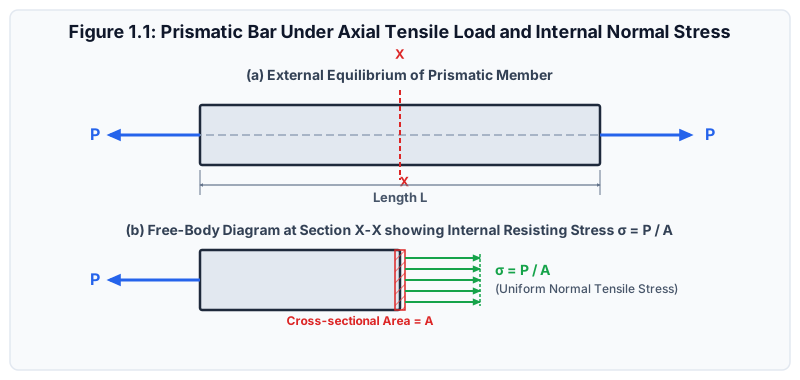
Civil Engineering Significance:
Near the point where a concentrated load is applied (or near a support reaction), the internal stress distribution is highly non-uniform and complex (local stress concentrations occur). However, at a cross-section situated at a distance equal to or greater than the largest cross-sectional dimension ( or ), the stress distribution becomes essentially uniform, and the simple formula holds with high accuracy.
3. Governing Mathematical Formulations & Derivations
3.1 The Cauchy Stress Tensor (3D State of Stress)
Consider an infinitesimal cube of dimensions excised from an arbitrary point within a stressed solid.
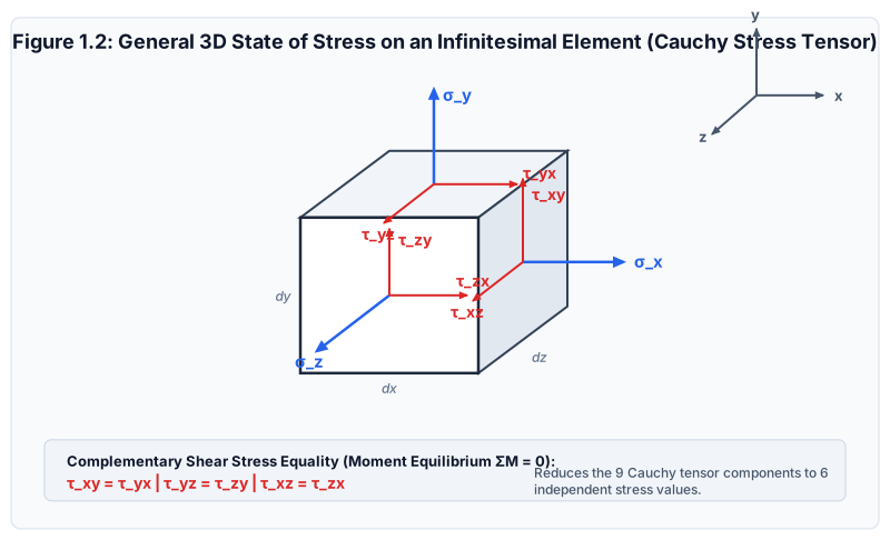
On each of the three orthogonal faces, one normal stress and two shear stresses act, giving 9 total stress components represented by the Cauchy Stress Tensor :
Subscript Convention for Shear Stresses ():
- First subscript (): The coordinate axis perpendicular to the plane on which the stress acts (the normal to the face).
- Second subscript (): The direction along which the shear stress acts.
3.2 Proof of Complementary Shear Stress Equality
To prove that , consider the rotational moment equilibrium of the infinitesimal 2D element (, unit depth ) about its centroid :
The forces produced by the normal stresses and pass symmetrically through the centroid and exert zero moment. The shear forces acting on the four faces create couples:
Canceling the non-zero volume element :
By identical moment equilibrium about the remaining two axes:
[!IMPORTANT] Cauchy's Complementary Shear Law: A shear stress on any plane is always accompanied by an equal, mutually perpendicular shear stress on the adjacent plane directed toward or away from their common corner. Consequently, the 3D stress tensor is symmetric, reducing the number of independent stress components from 9 to 6 ().
3.3 Mathematical Formulation of Shear Strain ()
Consider an infinitesimal rectangular plate element in the -plane having undeformed dimensions and .
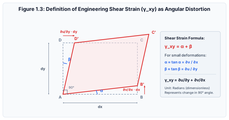
Under shear deformation:
- Fiber rotates through angle due to displacement gradient .
- Fiber rotates through angle due to displacement gradient .
For infinitesimal displacements, and :
The total angular distortion, defined as the Engineering Shear Strain (), is:
[!NOTE] In tensor mechanics, Tensorial Shear Strain is defined as . Tensorial shear strain transforms identically to normal strains via Mohr's circle of strain without requiring an extraneous factor of 2.
3.4 Engineering Stress-Strain vs True (Natural) Stress-Strain
In standard tension testing of structural metals:
- Engineering (Nominal) Stress (): where is the original, undeformed cross-sectional area.
- True Stress (): where is the instantaneous, actual cross-sectional area under load .
- Engineering Strain ():
- True (Hencky / Natural) Strain ():
Mathematical Interrelationship assuming Constant Volume:
Assuming plastic incompressibility (constant volume of metal during plastic deformation, ):
Substituting into the definition of True Stress:
[!WARNING] The relationships and are strictly valid only up to the onset of necking (ultimate tensile strength). After necking initiates, deformation becomes localized and non-uniform, rendering the constant-volume gauge assumption invalid.
4. Fundamental Assumptions & Limitations of Elastic Mechanics
All foundational derivations in linear elastic mechanics rely on four core idealizations:
- Homogeneity: The physical and mechanical properties of the material are identical at all spatial points ().
- Isotropy: The material properties are identical in all directions at any given point ().
- Continuum Hypothesis: Matter is continuously distributed throughout the region, neglecting discrete atomic lattices, dislocations, micro-voids, and grain boundaries.
- Infinitesimal Deformations (Small Strain Theory): Deformations and rotations are sufficiently small such that geometric equilibrium can be formulated using the undeformed initial dimensions of the structure.
5. Indian Standard (IS) Code Relevance
5.1 IS 456:2000 (Plain and Reinforced Concrete)
- Clause 38.1: The assumption that plane sections normal to the axis remain plane after bending requires linear distribution of normal strain across the cross-section.
- Table 21: Permissible shear stresses and bond stresses represent shear stress intensity limits derived directly from Cauchy's complementary shear mechanics.
5.2 IS 800:2007 (General Construction in Steel)
- Section 5 (Design Basis): Normal design yield strengths () are based on nominal engineering yield stress obtained from standard tensile testing per IS 1608 / ISO 6892.
6. Comparative Analysis
| Parameter | Engineering Formulation | True (Natural) Formulation |
|---|---|---|
| Area Used | Original cross-sectional area () | Instantaneous actual area () |
| Length Used | Original gauge length () | Instantaneous incremental length () |
| Tension Relationship | (since ) | |
| Compression Relationship | (since ) | |
| Magnitude of Strain | in tension | in tension |
| Additive Property | Not additive: | Strictly additive: |
| Primary Application | Structural design of buildings and bridges | Metal forming, plasticity, high-strain impact |
7. Step-by-Step Solved Numerical Examples
Example 1.1: Prismatic Tensile Bar with Independent Recalculation (SSC JE / State AE Level)
Problem Statement:
A solid circular mild steel tie rod of length and diameter is subjected to an axial tensile force of . Calculate:
- The nominal normal tensile stress () developed in the rod.
- The total elongation () if Young's modulus .
- The longitudinal engineering strain ().
Step-by-Step Solution:
-
Cross-Sectional Area ():
-
Normal Tensile Stress ():
-
Total Elongation (): Given , :
-
Engineering Longitudinal Strain ():
Independent Verification Check: (Verified exact match).
Example 1.2: True Stress vs Engineering Stress at High Strain (GATE CE Level)
Problem Statement:
A cylindrical tensile specimen of gauge length and initial diameter is loaded into the plastic region until its length reaches under a tensile load of . Assuming uniform plastic deformation with constant volume:
- Determine the nominal engineering stress () and nominal engineering strain ().
- Determine the actual cross-sectional area at this load.
- Calculate the true stress () and true strain ().
Step-by-Step Solution:
-
Initial Area ():
-
Engineering Strain ():
-
Engineering Stress ():
-
Instantaneous Actual Area (): By volume conservation ():
-
True Stress (): Direct calculation from actual area:
Check using analytical formula:
-
True Strain ():
Observation: The true stress () is higher than the nominal engineering stress () because the load-bearing cross-section has shrunk by .
Example 1.3: Shear Stress and Angular Distortion in a Rubber Bearing Pad (UPSC ESE Level)
Problem Statement:
An elastomeric bridge bearing pad of rectangular plan dimensions and thickness is subjected to a horizontal shear force of caused by bridge deck thermal expansion. The shear modulus of the elastomer is .
- Find the average shear stress () acting on the bearing face.
- Calculate the resulting horizontal lateral displacement () of the top surface relative to the bottom surface.
- Determine the engineering shear strain ().
Step-by-Step Solution:
-
Shear Area (): The shear force acts parallel to the horizontal surface:
-
Average Shear Stress ():
-
Engineering Shear Strain (): Applying Hooke's Law in shear ():
-
Horizontal Lateral Displacement (): From geometric definition of shear distortion ():
Independent Recalculation Check:
8. Common Pitfalls & Competitive Exam Traps
[!WARNING] Trap 1: Confusing Tensorial Strain with Engineering Strain
In GATE Numerical Answer Type (NAT) problems, pay close attention to whether the question asks for Engineering Shear Strain () or Tensorial Shear Strain ().
Remember: . Forgetting the factor of is responsible for frequent lost marks!
[!WARNING] Trap 2: Applying Engineering Relations into Post-Necking Regimes
In UPSC ESE Conventional papers, students often write for fracture points. This formula is strictly invalid once localized necking begins, because deformation is no longer uniform along the gauge length.
[!WARNING] Trap 3: Unit Mixing in Stress Calculations
When calculating stress with force in kilonewtons () and dimensions in meters (), yields (which is ), NOT !
Rule of thumb: Always convert force to and lengths to to directly obtain stress in .
9. Quick Revision Formula Box
10. References & Source Literature
- Timoshenko, S. P., & Gere, J. M. (1972). Mechanics of Materials, Van Nostrand Reinhold Company, New York.
- Gere, J. M., & Goodno, B. J. (2018). Mechanics of Materials, 9th Edition, Cengage Learning, Boston.
- Punmia, B. C., Jain, A. K., & Jain, A. K. (2017). Mechanics of Materials, 15th Edition, Laxmi Publications, New Delhi.
- Bureau of Indian Standards (2000). IS 456:2000 — Plain and Reinforced Concrete - Code of Practice, New Delhi.
- Bureau of Indian Standards (2007). IS 800:2007 — General Construction in Steel - Code of Practice, New Delhi.