Bending Stresses in Beams (04_bending_stresses_in_beams)
Difficulty Level
Intermediate to Advanced
Target Examinations
GATE CE, UPSC ESE, SSC JE, State AE/JE, RRB JE
Primary Prerequisites
Pure Bending Theory (SOM-04-01), Section Modulus (SOM-04-02), Centroid & Parallel Axis Theorem
Benchmark Formulas
Modular ratio m=E2E1; Transformed width beq=m⋅b1; Stress ratio σ2σ1=m; Transformed MOI Itr=I2+mI1; Capacity Msafe=min(σallow,2y2Itr,mσallow,1y1Itr)
Authoritative Code References
IS 456:2000 (Annex B, Cl. B-1.3, B-2.1), IS 800:2007 (Cl. 8.2), IS 3629:1986, IRC:22-2015
2. Physical Mechanics & Theoretical Foundation
In structural engineering, a composite beam (or flitched beam) is a flexural member built by rigidly connecting two or more distinct materials (such as timber and structural steel, or concrete and reinforcing steel bars) to act as a single monolithic unit under bending.
                    ┌─────── b ───────┐
                 ───┼─────────────────┼───
                ▲   │  Steel Plate    │   Material 1 (E₁, σ₁)
                │   ├─────────────────┤
                d   │                 │
                │   │  Timber Core    │   Material 2 (E₂, σ₂)
                │   ├─────────────────┤
                ▼   │  Steel Plate    │   Material 1 (E₁, σ₁)
                 ───┼─────────────────┼───
                    └─────────────────┘
2.1 The Engineering Need for Flitched Beams
Deflection Control & Headroom Optimization: In architectural floor framing and timber bridge decks, timber joists often lack sufficient flexural stiffness (EI), leading to excessive serviceability deflections or requiring excessively deep sections that intrude on vertical clearance. Bolting high-modulus structural steel flitch plates to timber drastically amplifies flexural rigidity without increasing overall floor depth.
Economic Efficiency: Structural steel provides high tensile and compressive strength (Es≈200 GPa, fy≥250 MPa), while timber provides lightweight bulk volume and lateral stability at a fraction of the cost (Ew≈10−14 GPa).
Heritage Restoration & Retrofitting: Decayed or under-designed historic timber girders are routinely strengthened in situ by sandwiching them between mild steel flitch plates secured by through-bolts.
2.2 Kinematic Compatibility vs Stress Discontinuity
The mechanics of composite flexure rests on two governing principles:
Kinematic Strain Compatibility (Euler-Bernoulli Hypothesis):
Assuming perfect bond (no interfacial slip between materials):
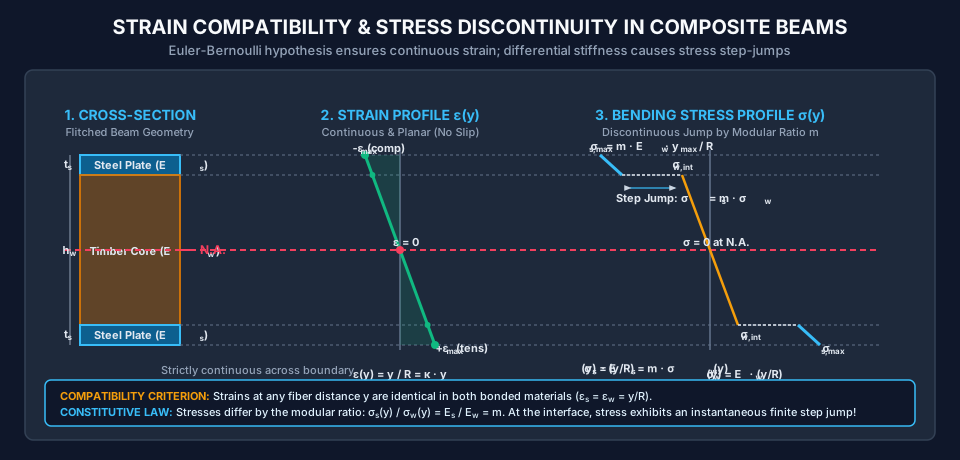
ϵ1(y)=ϵ2(y)=Ry=κ⋅y
The longitudinal normal strain varies continuously and linearly across the entire cross-section from the neutral axis (y=0).
Constitutive Stress Discontinuity:
Because the materials have different moduli of elasticity (E1=E2), Hooke's law dictates:
σ1(y)=E1ϵ(y)=E1(Ry)σ2(y)=E2ϵ(y)=E2(Ry)
Taking the ratio of stresses at the exact same distance y from the neutral axis:
σ2(y)σ1(y)=E2E1=m
where m is the modular ratio. At the physical boundary separating the two bonded materials, the strain is identical, but the normal stress exhibits an abrupt, instantaneous step jump by a factor equal to m.
3. Mathematical Derivations & Governing Equations
3.1 The Transformed Section Concept (Equivalent Area Method)
To analyze a multi-material composite section using elementary homogeneous beam formulas (σ=My/I), we transform the composite section into an equivalent fictitious section composed entirely of a single base material (typically Material 2, the weaker material such as timber or concrete).
1. Internal Force Equivalence:
Consider an infinitesimal element of area dA1 of Material 1 located at distance y from the neutral axis. The internal normal force carried by this element is:
dF1=σ1dA1=(mσ2)dA1=σ2(mdA1)
This demonstrates that the internal force carried by area dA1 of Material 1 is identical to the force carried by an equivalent area dA2′ of Material 2, provided:
dA2′=m⋅dA1
2. The Direction of Geometric Transformation:
Because the normal stress depends strictly on the vertical coordinate y (σ∝y), replacing dA1 with mdA1must not alter the distance y from the neutral axis.
Therefore:
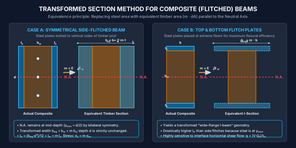
The vertical dimension (depth d) must remain strictly unchanged.
The horizontal dimension (width b) must be multiplied by the modular ratio m:
beq=m⋅b1
Fundamental Rule of Transformation:
Always scale widths parallel to the neutral axis; never alter dimensions perpendicular to the neutral axis.
3.2 Neutral Axis of Transformed Section
For unsymmetrical composite beams (e.g., steel plate on one side or bottom only), the neutral axis corresponds to the centroid of the transformed equivalent section.
Taking a reference datum line at the extreme base fiber:
yˉ=∑Atr,i∑Atr,iyi=A2+mA1A2y2+mA1y1
where:
A2,y2 are the area and centroidal height of the base material.
A1,y1 are the area and centroidal height of the reinforcement.
m=E1/E2 is the modular ratio.
3.3 Transformed Second Moment of Area (Itr)
The moment of inertia of the transformed section about its centroidal neutral axis is computed using the parallel axis theorem:
Critical Design Principle:
Whichever material reaches its allowable stress first under an increasing moment dictates the structural capacity of the composite member.
When a composite beam flexes under vertical shear force V, horizontal shear stresses develop along the bonded interface between the steel and timber.
1. Horizontal Shear Flow (q):
q=ItrVQ1′
where:
V is the transverse shear force at the section.
Q1′ is the first moment of area of the transformed attached component about the neutral axis:
Q1′=(mA1)⋅d1
Itr is the total transformed moment of inertia.
2. Interface Shear Stress (τint):
τint=bintq=ItrbintVQ1′
where bint is the physical contact contact width at the interface.
3. Bolt Pitch (Spacing p):
If the connection is made via through-bolts having a shear capacity (single or double shear) Rv:
p≤qn⋅Rv=VQ1′n⋅Rv⋅Itr
where n is the number of bolts provided at each longitudinal pitch cross-section.
4. Engineering Assumptions & Validity Limits
Perfect Interfacial Bond (No Slip): The adhesive, weld, or bolting system provides full strain compatibility at the interface without slip (Δuslip=0).
Linear Elastic Behavior: Both materials obey Hooke's law up to their respective permissible stresses (σ1≤σallow,1 and σ2≤σallow,2).
Euler-Bernoulli Hypothesis: Cross-sections remain plane and perpendicular to the neutral axis throughout bending.
Equal Curvature: Both components bend to the exact same radius of curvature R along their bonded length (1/R1=1/R2=1/R).
No Local Buckling: Steel flitch plates under compression are sufficiently thick or continuously restrained against out-of-plane buckling by through-bolts conforming to IS 800:2007 limits.
The diagram below illustrates the physical multi-material section alongside its equivalent transformed section in terms of timber base material.
Figure 2: Strain Compatibility vs Stress Discontinuity
The diagram below compares the continuous linear strain profile ϵ(y) with the discontinuous stepped bending stress distribution σ(y) across the timber-steel boundary.
6. Solved Numerical Examples (Python-Verified)
Example 1: Symmetrical Side-Flitched Timber Joist
Problem Statement:
A timber flitched beam is formed by sandwiching a sal wood joist of width bw=150.0 mm and depth d=300.0 mm between two mild steel plates of thickness ts=12.0 mm each and depth 300.0 mm. The plates are securely bolted on both vertical faces over the full depth.
The modular ratio between steel and timber is m=EwEs=20.0.
The permissible flexural stress in timber is σallow,w=10.0 N/mm2 and in steel is σallow,s=140.0 N/mm2.
Compute the second moment of area of the transformed section in terms of equivalent timber (Itr).
Determine which material reaches its allowable stress first, and find the safe bending moment capacity (Msafe) of the flitched beam.
Calculate the moment capacity of the unreinforced timber beam alone, and evaluate the percentage strength gain provided by the steel flitch plates.
Solution:
Step 1: Transformed Cross-Sectional Geometry:
By symmetry, the neutral axis lies at mid-depth:
ymax=2d=2300.0=150.0 mm
Total physical width of steel:
bs=2×ts=2×12.0=24.0 mm
Transformed equivalent width of steel in terms of timber:
Step 2: Allowable Stress & Governing Capacity:
Both timber and steel extreme fibers are located at y=150.0 mm.
If timber reaches its allowable stress σw=10.0 N/mm2:
σs=m⋅σw=20.0×10.0=200.0 N/mm2
Since 200.0 N/mm2>σallow,s=140.0 N/mm2, steel is overstressed!
Therefore, steel governs the design:
Maximum allowable stress in steel is σs=140.0 N/mm2.
Corresponding stress induced in the adjacent timber extreme fiber:
Adding just 24 mm total width of steel plates (13.8% increase in cross-sectional area) increases moment capacity by nearly triple (2.94×)!
Example 2: Top and Bottom Flitch Plates (Symmetrical I-Shaped Transformation)
Problem Statement:
A timber beam b=200.0 mm wide and hw=300.0 mm deep is strengthened by bonding two structural steel plates of dimensions 200.0 mm wide by ts=15.0 mm thick to its top and bottom horizontal faces. Total overall beam depth is D=300.0+2(15.0)=330.0 mm.
Given: m=Es/Ew=15.0, σallow,w=8.0 N/mm2, σallow,s=120.0 N/mm2.
Compute the transformed moment of inertia Itr about the neutral axis.
Determine the safe bending moment capacity Msafe.
If the beam is subjected to a service moment M=60.0 kNm, calculate the maximum tensile stress in steel and the maximum compressive stress in timber.
Solution:
Step 1: Transformed Moment of Inertia Itr:
By symmetry, the neutral axis is at mid-depth (y=0 at center of timber core).
Steel Plates (Two plates, each 200×15 mm, centroid at y=±157.5 mm):
Is,own=2×(12bts3)=2×(12200.0×15.03)=2×56,250=112,500.0 mm4Is,d2=2×[As⋅(2hw+ts)2]=2×[(200.0×15.0)×(157.5)2]=2×[3000×24,806.25]=148.8375×106 mm4Is=Is,own+Is,d2=0.1125×10⁶+148.8375×106=148.950×106 mm4
Transformed moment of inertia in terms of timber (m=15.0):
Problem Statement:
A timber joist b=120.0 mm wide and hw=200.0 mm deep is reinforced on its bottom tension face only with a single structural steel plate 120.0 mm wide and ts=10.0 mm thick. Total beam depth is 210.0 mm.
Given: Modular ratio m=20.0.
Allowable stresses:
Timber in compression: σallow,w,c=10.0 N/mm2
Timber in tension: σallow,w,t=6.0 N/mm2
Steel in tension: σallow,s,t=140.0 N/mm2
Locate the centroidal neutral axis of the transformed section measured from the bottom of the steel plate.
Determine the transformed moment of inertia Itr about the neutral axis.
Calculate the safe sagging bending moment capacity Msafe.
For a transverse vertical shear force V=20.0 kN, calculate the horizontal shear flow q (in N/mm) and the horizontal shear stress τint acting at the timber-steel interface.
Solution:
Step 1: Neutral Axis Depth (yˉ from bottom of steel plate):
Steel plate area: As=120.0×10.0=1,200.0 mm2
Transformed steel area: As,tr=mAs=20.0×1,200.0=24,000.0 mm2
Centroid of steel from bottom: ys=210.0=5.0 mm
Timber joist area: Aw=120.0×200.0=24,000.0 mm2
Centroid of timber from bottom: yw=10.0+2200.0=110.0 mm
Taking moments of transformed areas about bottom datum (y=0):
yˉbot=As,tr+AwAs,trys+Awyw=24,000.0+24,000.0(24,000.0×5.0)+(24,000.0×110.0)yˉbot=48,000.0120,000.0+2,640,000.0=48,000.02,760,000.0=57.50 mm
Distance from neutral axis to top extreme timber fiber:
yˉtop=(hw+ts)−yˉbot=210.0−57.50=152.50 mm
Distance from neutral axis to timber-steel interface:
yint=yˉbot−ts=57.50−10.0=47.50 mm(below NA)
Step 2: Transformed Moment of Inertia (Itr):
Using the parallel axis theorem on both components:
Governing Failure Mode: The beam is governed by compressive crushing of timber at the top extreme fiber (M=13.93 kNm) because shifting the neutral axis downward (57.5 mm from bottom) placed the top fiber at a large distance of 152.5 mm from the neutral axis!
Step 4: Interfacial Shear Flow and Shear Stress under V=20.0 kN:
First moment of area of the transformed steel plate about the neutral axis:
7. Engineering Applications & Real-World Case Studies
Reinforced Concrete Beams (Working Stress Method - IS 456:2000 Annex B):
The elastic analysis of RC beams is the most widespread application of the modular ratio method. Concrete in tension is assumed cracked (Ec,t=0), and tensile steel bars (Ast) are replaced by an equivalent concrete area m⋅Ast placed at effective depth d. The neutral axis depth x is found by setting first moments of areas equal: 2bx2=mAst(d−x).
Timber Floor Reinforcement in Historic Renovation (IS 3629 / Eurocode 5):
Heritage masonry structures with sagged timber floor joists are strengthened by sandwiching existing wood members between vertical mild steel plates secured by high-strength through-bolts, restoring structural integrity without dismantling decorative plaster ceilings below.
Steel-Concrete Composite Bridge Girders (IRC:22-2015 / IS 11384):
Highway viaducts utilize rolled steel plate girders connected to an in-situ cast reinforced concrete deck slab via headed shear studs. The transformed section method with modular ratio m=Es/Ec allows bridge designers to calculate longitudinal flexural stresses under dead load and IRC Class A/70R live vehicle axle trains.
Bimetallic Thermostatic Strips in Mechanical Sensors:
Bonded strips of two metals with differing coefficients of thermal expansion and Young's moduli flex into an arc when heated, closing or opening electrical circuits in thermostats and fire alarms according to composite beam mechanics.
8. Comparative Analysis & Summary Matrix
Feature
Symmetrical Side Flitch Plates
Top & Bottom Flitch Plates
Unsymmetrical Single Plate (Bottom Only)
Physical Geometry
Plates bolted to vertical side faces
Plates bonded to horizontal faces
Plate bonded to bottom tension face
Neutral Axis Position
Strictly at mid-depth (ymax=d/2)
Strictly at mid-depth (ymax=D/2)
Shifted downward toward steel plate (yˉ<d/2)
Transformed Section Shape
Solid rectangular section (beq×d)
Wide-flange I-shaped section
Asymmetrical T-shaped section
Flexural Efficiency (η)
Moderate (≈0.33)
Very High (≥0.60)
High for tension-weak materials
Steel Stress Location
Extreme steel fiber is at d/2
Extreme steel fiber is at D/2>d/2
Extreme steel fiber is at bottom distance yˉ
Fabrication Complexity
Simple (standard through-bolts)
Requires adhesive bond or countersunk screws
Common in RC repair (CFRP/Steel bottom plate)
Interfacial Shear Risk
Moderate; through-bolts clamp sides
High; horizontal shear flow q=VQ/I
Very High; prone to plate end peeling
9. Key Takeaways & Exam-Oriented Mnemonics
The Width-Only Rule:
Always scale dimension parallel to the neutral axis: beq=m⋅b. Never scale depth d!
The Stress Jump Rule:
At the boundary between two materials:
σstiffer=m⋅σweakerStrain is continuous; stress is discontinuous!
Allowable Capacity Determination:
Never assume which material governs beforehand. Calculate:
M1=(mσallow,1)y1Itr,M2=σallow,2y2Itr
The smaller moment controls the design.
Top/Bottom Flitch Superiority:
For the same volume of steel, top and bottom plates produce a much higher transformed moment of inertia than side plates because I∝A⋅d2 (parallel axis effect).
10. Common Pitfalls, Traps & Misconceptions
[!WARNING]
Pitfall 1: Transforming Depth Instead of Width
Transforming depth (deq=m⋅d) changes the lever arm y and generates an incorrect moment of inertia (I∝d3⟹m3 error!). Width must be transformed (beq=m⋅b), preserving the linear strain gradient.
[!CAUTION]
Pitfall 2: Forgetting to Multiply Timber Stress by m to Get Steel Stress
When evaluating stress using Itr (in timber units), the formula σ=My/Itr gives the stress in timber. To find the actual physical stress in steel, you must multiply by the modular ratio: σs=m⋅(My/Itr).
[!NOTE]
Pitfall 3: Neglecting Neutral Axis Shift in Unsymmetrical Sections
Adding a steel plate to the bottom of a timber joist shifts the neutral axis downward. The top extreme fiber of timber is now at a significantly greater distance from the neutral axis than before (yˉtop>d/2). Consequently, compressive stress in timber increases and often becomes the governing failure mode!
11. Standard Specifications & Code Provisions
Standard
Clause / Section
Engineering Requirement
IS 456:2000
Annex B, Cl. B-1.3
Modular Ratio in RC Design:m=3σcbc280, where σcbc is permissible compressive stress in concrete in bending. The factor 3 accounts for long-term creep and shrinkage of concrete under sustained dead load.
IS 456:2000
Annex B, Cl. B-2.1
Transformed Crack Section: For flexural analysis under working loads, concrete in tension is ignored, and steel area is replaced with equivalent concrete area mAst. For compression steel, equivalent area is (1.5m−1)Asc to account for creep.
IS 800:2007
Cl. 8.2 & Cl. 10
Fastener Pitch in Built-Up Beams: Longitudinal pitch of bolts or intermittent welds connecting flitch plates must resist horizontal shear flow q=VQ/I. Pitch p≤16t or 200 mm (tension), and ≤12t or 200 mm (compression) to prevent plate buckling.
IS 3629:1986
Cl. 6.4
Composite Timber Construction: Permissible bending stresses and moisture contents for structural timber when combined with steel plates; recommends modular ratios m=15−20 for Group A/B Indian timbers.
IRC:22-2015
Cl. 605
Composite Road Bridges: Specifies modular ratios for short-term and long-term load combinations in steel girder concrete deck composite highway superstructures.
12. Comprehensive Formula Box & Practice Problems
Governing Formula Summary
Modular Ratio: m=E2E1(E1>E2)Transformed Equivalent Width: beq=m⋅b1(Depth d unchanged)Neutral Axis Datum Height: yˉ=∑Atr,i∑Atr,iyi=A2+mA1A2y2+mA1y1Transformed Moment of Inertia: Itr=I2+mI1=∑(Itr,own+Atrd2)Bending Stresses: σ2(y)=ItrMy,σ1(y)=m⋅σ2(y)=m(ItrMy)Safe Moment Capacity: Msafe=min(σallow,2ymax,2Itr,mσallow,1ymax,1Itr)Horizontal Shear Flow: q=ItrVQ1′,Bolt Pitch: p≤qnRv
Practice Problems
(GATE CE Pattern) A composite bar is constructed from two materials with elastic moduli E1=200 GPa and E2=100 GPa. If the beam is bent into a circular arc of radius R=25 m, what is the ratio of the longitudinal bending stress in material 1 to material 2 at the exact same distance y=50 mm from the neutral axis?
(A) 1.0
(B) 2.0
(C) 0.5
(D) 4.0
Answer: (B) 2.0. By strain compatibility, ϵ1=ϵ2=y/R. Therefore, σ1/σ2=(E1ϵ)/(E2ϵ)=E1/E2=200/100=2.0.
(UPSC ESE Pattern) In the transformed section method for a flitched beam composed of wood and steel with modular ratio m=Es/Ew:
(A) The depth of steel is multiplied by m
(B) The width of steel is multiplied by m
(C) Both depth and width of steel are multiplied by m
(D) Both depth and width of steel are multiplied by m
Answer: (B). The transformation must scale dimensions parallel to the neutral axis (width) to preserve the linear vertical strain gradient ϵ(y)∝y.
(State AE Pattern) A wooden beam 100 mm wide and 150 mm deep is reinforced with two steel plates 10 mm thick and 150 mm deep on its sides. If m=20, the equivalent width of a purely wooden beam having the same flexural stiffness is:
(A) 300 mm
(B) 400 mm
(C) 500 mm
(D) 200 mm
Answer: (C) 500 mm. Total width of steel bs=2×10=20 mm. Equivalent width beq=bw+m⋅bs=100+20(20)=100+400=500 mm.