Columns under Biaxial Bending (Bresler's Formulations & Analysis)
In this chapter (4 topics)
On this page
- 1. Introduction and Architectural Overview
- 2. Physical Mechanics & Inclined Neutral Axis Geometry
- 2.1 The Inclined Neutral Axis
- 2.2 Three-Dimensional Equilibrium Equations
- 3. The 3D Interaction Failure Surface (Pu - Mux - Muy)
- 4. Bresler's Load Contour Method (IS 456:2000 Clause 39.6)
- 4.1 Evaluation of the Exponent αn
- 4.2 Physical Meaning of the αn Variation
- 5. Pure Concentric Axial Capacity Puz vs Short Column Capacity Pu
- 5.1 Critical Distinction: Clause 39.6 (Puz) vs Clause 39.3 (Pu)
- 6. Bresler's Reciprocal Load Method
- 6.1 Structural Design Criterion
- 6.2 Validity Bounds and Limitations
- 7. Step-by-Step Structural Design Procedure per IS 456 & SP 16
- Step 1: Factored Design Actions and Minimum Eccentricities
- Step 2: Section Dimensions and Steel Trial
- Step 3: Determine Uniaxial Capacities Mux1 and Muy1
- Step 4: Calculate Concentric Capacity Puz
- Step 5: Compute Axial Ratio and Interaction Exponent αn
- Step 6: Verify Interaction Criterion
- 8. Detailed Engineering Diagrams & Visual Walkthrough
- Figure 1: 3D Interaction Failure Surface & Bresler Load Contours
- Figure 2: Variation of Exponent αn, Puz Formulation & Reciprocal Method
- 9. Pre-Calculated Solved Numerical Examples
- Problem 1: Structural Verification of a Column Section under Biaxial Bending (Load Contour Method)
- Problem 2: Evaluation of Column Capacity using Bresler's Reciprocal Load Method
- Problem 3: Determination of Permissible Biaxial Moment for Given Axial Force
- 10. Comprehensive Comparison Table: Methods of Biaxial Analysis
- 11. Practical Detailing and Common Site Pitfalls
- 12. Competitive Examination Traps & Quick Formula Sheet
- Common Exam Traps
- Master Formula Sheet
- 13. Practice Problems
- Problem 1 (GATE CE Format - NAT)
- Problem 2 (UPSC ESE Format - Multiple Choice)
- Problem 3 (State AE / SSC JE Format)
1. Introduction and Architectural Overview
In actual reinforced concrete framing systems—such as building corner columns, columns supporting spatial space frames, bridge piers subjected to longitudinal braking and transverse wind/seismic forces, and columns framing into orthogonal two-way beams—columns are rarely subjected to pure axial compression or uniaxial bending alone. Instead, they are subjected to an axial compression force acting simultaneously with bending moments about both principal centroidal axes ( about the major axis and about the minor axis).
Equivalently, this state of stress can be represented as an axial compression force acting with biaxial eccentricities:
                           Y
                           ▲
                           │        • P_u (e_x, e_y)
                           │       ┌────────┐
                           │       │        │
                           │   e_y │        │
                           │◄─────►│        │
                     ──────┼───────┴────────┼──────► X
                           │         e_x    │
                           │◄──────────────►│
                           │                │
                           │                │
                           │                │
                           ▼
When a column is subjected to biaxial bending, the neutral axis does not lie parallel to either principal axis; it is inclined at an angle across the section. The resulting compressive stress zone is triangular, trapezoidal, or pentagonal at a corner of the cross-section. Direct numerical integration of concrete compression and discrete rebar stresses for every arbitrary angle and neutral axis depth is computationally prohibitive for routine manual design.
To solve this problem, IS 456:2000 (Clause 39.6) incorporates Bresler's Load Contour Method, an interaction formulation that relates the biaxial moments to the corresponding uniaxial moment capacities under the same axial load . In addition, Bresler's Reciprocal Load Method provides an alternative interaction equation based on uniaxial axial capacities and the pure concentric axial capacity .
2. Physical Mechanics & Inclined Neutral Axis Geometry
2.1 The Inclined Neutral Axis
Under uniaxial bending about the axis, the strain profile varies only in the -direction (), producing a rectangular concrete compression block. Under biaxial bending, the strain distribution varies linearly across the 2D plane:
The neutral axis is defined by the locus of points where :
Where:
- is the inclination of the neutral axis with respect to the axis.
- is the intercept on the -axis.
2.2 Three-Dimensional Equilibrium Equations
At the ultimate limit state of collapse, the internal stresses must balance the external factored actions:
- Axial Force Equilibrium:
- Moment Equilibrium about Axis:
- Moment Equilibrium about Axis:
Because concrete stress follows the parabolic-rectangular IS 456 stress block perpendicular to the inclined neutral axis, evaluating the double integrals requires dividing the compressive area into triangular or polygonal sub-elements. This rigorous approach is utilized in non-linear finite element software, but for design offices and competitive examinations, codified interaction methods are essential.
3. The 3D Interaction Failure Surface ()
The locus of all combinations of ultimate axial load and orthogonal moments that cause structural failure of a given reinforced concrete cross-section forms a continuous, smooth, convex three-dimensional surface in Cartesian space :
- Top Apex ():
- Represents pure concentric axial compression capacity .
- Bottom Apex ():
- Represents pure axial tensile capacity governed solely by reinforcement: .
- Principal Planes:
- The intersection of the 3D surface with the plane () generates the classical uniaxial interaction diagram for bending about the axis.
- The intersection with the plane () generates the uniaxial interaction diagram for bending about the axis.
- Horizontal Slices at Constant :
- A horizontal cutting plane at any design axial force intersects the 3D surface to form a closed convex curve known as an interaction load contour in the coordinate plane.
- The intercepts of this contour on the coordinate axes are (at ) and (at ).
4. Bresler's Load Contour Method (IS 456:2000 Clause 39.6)
Boris Bresler (1960) approximated the family of horizontal interaction load contours by a non-dimensional power equation:
Where:
- = applied factored design moments about the and axes respectively, including the effects of minimum accidental eccentricity ( and ).
- = maximum uniaxial moment capacity of the column under the design axial load bending solely about the axis ().
- = maximum uniaxial moment capacity of the column under the design axial load bending solely about the axis ().
- = an interaction exponent that depends on the axial load ratio .
4.1 Evaluation of the Exponent
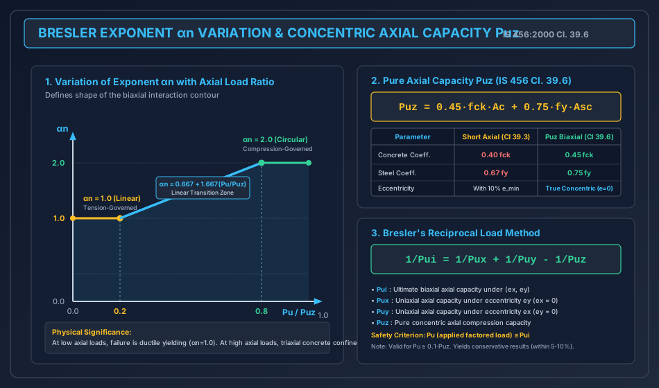
In IS 456:2000 (Clause 39.6), the exponent is a function of the normalized axial force ratio :
   α_n
    ▲
2.0 ┼───────────────────────┌────────────────── (α_n = 2.0, Circular/Elliptic)
    │                      /│
    │                     / │
    │                    /  │
    │                   /   │   Linear Transition:
    │                  /    │   α_n = 0.667 + 1.667(P_u / P_uz)
1.0 ┼─────────────────┘     │
    │ (α_n = 1.0, Straight) │
    │                       │
  0 ┴─────────┬─────────────┴────────┬─────────► P_u / P_uz
    0        0.2           0.8      1.0
4.2 Physical Meaning of the Variation
- At Low Axial Loads ():
- The member behaves essentially as a flexural beam-column dominated by ductile steel yielding (tension failure).
- In tension-controlled sections, yielding along one edge rapidly limits moment capacity in the other direction, leading to a linear interaction (, a straight-line diagonal contour).
- At High Axial Loads ():
- The member is in heavy compression. Concrete crushing governs without rebar yielding.
- Triaxial confinement of the core allows a spherical/elliptical failure surface (), significantly bulging outwards and expanding the safe zone.
- In the Transition Zone ():
- The failure mode transitions from tension yielding to compression crushing. The exponent increases linearly from to .
5. Pure Concentric Axial Capacity vs Short Column Capacity
The denominator used in computing the axial force ratio is defined in IS 456:2000 Clause 39.6 as:
Where:
- is the net area of concrete.
- is the total cross-sectional area of longitudinal column reinforcement.
- is the characteristic compressive cube strength of concrete.
- is the characteristic yield strength of longitudinal reinforcement.
5.1 Critical Distinction: Clause 39.6 () vs Clause 39.3 ()
A ubiquitous trap in competitive examinations is confusing with the short column axial capacity from Clause 39.3:
| Structural Parameter | Clause 39.3 ( for Short Axial Column) | Clause 39.6 ( Pure Concentric Capacity) |
|---|---|---|
| Mathematical Expression | ||
| Concrete Stress Factor | ( reduction from ) | (, unreduced) |
| Steel Stress Factor | ( reduction from ) | () |
| Eccentricity Assumption | Accounts for mandatory accidental eccentricity | True concentric loading () |
| Application | Safe load for column designed as axially loaded | Reference normalizing base for biaxial bending () |
| Numerical Ratio | Base capacity () |
[!IMPORTANT] Never substitute into the ratio ! You must calculate the unreduced concentric capacity .
6. Bresler's Reciprocal Load Method
In 1960, Boris Bresler also proposed an approximate method based on reciprocal axial loads. Approximating the 3D failure surface by an oblique plane intersecting the coordinate planes at and , the interaction is given by:
Where:
- = ultimate axial capacity of the column under biaxial eccentricities .
- = ultimate axial capacity under uniaxial eccentricity with (bending about major axis only).
- = ultimate axial capacity under uniaxial eccentricity with (bending about minor axis only).
- = ultimate axial capacity under pure concentric axial load ().
6.1 Structural Design Criterion
For safety against collapse under factored axial force :
6.2 Validity Bounds and Limitations
- Axial Load Range: The reciprocal method is valid and accurate when . When axial compression is very small (), the reciprocals blow up towards infinity, leading to numerical instability and unconservative results.
- Accuracy: Extensive experimental testing indicates that Bresler's reciprocal load method is generally conservative, agreeing within to of experimental failure loads for normal column proportions.
- Application in Codes: While IS 456 officially codifies the Load Contour Method (Clause 39.6), the Reciprocal Load Method is widely accepted in international design (such as ACI 318) and frequently tested in competitive examinations (GATE CE and UPSC ESE).
7. Step-by-Step Structural Design Procedure per IS 456 & SP 16
When designing or verifying a reinforced concrete column under combined axial load and biaxial bending:
Step 1: Factored Design Actions and Minimum Eccentricities
Given factored axial force and factored bending moments and :
- Calculate statutory minimum eccentricities (IS 456 Clause 25.4):
- Determine governing design moments:
Step 2: Section Dimensions and Steel Trial
Assume trial cross-section dimensions and a symmetrical longitudinal reinforcement layout (e.g., 8 bars arranged symmetrically on 4 faces).
- Gross concrete area:
- Total steel area: (with )
- Net concrete area:
Step 3: Determine Uniaxial Capacities and
Using SP 16 interaction charts for the given steel distribution, concrete grade , and steel grade :
- For Bending about Axis:
- Axial load parameter:
- Reinforcement parameter:
- Cover ratio:
- Read flexural parameter from the appropriate chart .
- For Bending about Axis:
- Axial load parameter:
- Reinforcement parameter:
- Cover ratio:
- Read flexural parameter from the appropriate chart .
Step 4: Calculate Concentric Capacity
Step 5: Compute Axial Ratio and Interaction Exponent
- If
- If
- If
Step 6: Verify Interaction Criterion
Evaluate the left-hand side of Bresler's contour equation:
- If SAFE.
- If UNSAFE (increase section size or percentage of reinforcement ).
8. Detailed Engineering Diagrams & Visual Walkthrough
Figure 1: 3D Interaction Failure Surface & Bresler Load Contours
The diagram below illustrates the 3D convex failure surface in space, a section subjected to an inclined neutral axis at angle , and the resulting normalized Bresler load contours for various values of .
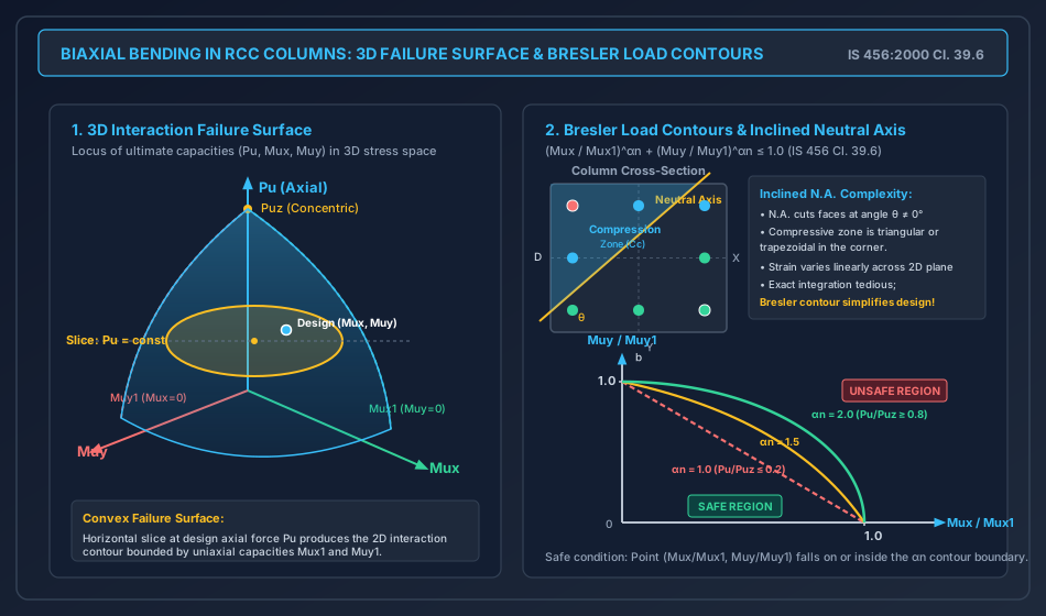
Figure 2: Variation of Exponent , Formulation & Reciprocal Method
The diagram below details the variation of with , the comparison between Clause 39.3 and Clause 39.6 axial formulations, and Bresler's Reciprocal Load Method.
9. Pre-Calculated Solved Numerical Examples
Problem 1: Structural Verification of a Column Section under Biaxial Bending (Load Contour Method)
Statement: A rectangular short column of cross-section is reinforced with 8 bars of diameter distributed equally on four faces, with an effective cover of to the bar center. The materials used are M25 grade concrete () and Fe 415 grade steel (). The column is subjected to a factored axial force and factored design moments and . Verify the adequacy of the section per IS 456:2000 Clause 39.6.
Solution:
Step 1: Geometric and Material Properties
- Breadth , Depth
- Gross area
- Longitudinal reinforcement: :
- Percentage of steel:
- Net concrete area:
- Effective cover :
Step 2: Calculate Pure Concentric Axial Capacity
According to IS 456:2000 Clause 39.6:
Step 3: Determine Axial Ratio and Exponent
Since , is in the linear transition regime:
Step 4: Determine Uniaxial Moment Capacities and
-
Capacity (Bending about Axis, ):
- From SP 16 Chart 44 (equal reinforcement on 4 faces, Fe 415, ):
-
Capacity (Bending about Axis, Depth , Width ):
- Interpolating between SP 16 Chart 44 () and Chart 45 ():
Step 5: Verify Interaction Formula
Applied moments: .
Conclusion: Since the interaction index , the column section is SAFE under the applied biaxial bending and axial load.
Problem 2: Evaluation of Column Capacity using Bresler's Reciprocal Load Method
Statement: A square column of size constructed with M30 concrete () and Fe 500 steel () has a longitudinal reinforcement area . Under an axial load, the eccentricities are and . From uniaxial interaction analysis:
- The uniaxial axial capacity with eccentricity () is .
- The uniaxial axial capacity with eccentricity () is . Using Bresler's Reciprocal Load Method, determine the maximum permissible biaxial axial load that the column can support. Check if an applied factored load is safe.
Solution:
Step 1: Pure Concentric Capacity
- Gross area
Step 2: Apply Bresler's Reciprocal Formula
Compute each reciprocal term:
Substitute into the reciprocal equation:
Step 3: Check Safety under Applied Load
- Applied factored load
- Ultimate biaxial capacity
- Demand-to-capacity ratio:
- Check validity bound: Since , the reciprocal method is fully valid.
Conclusion: The column is SAFE under the applied load (, with a reserve margin).
Problem 3: Determination of Permissible Biaxial Moment for Given Axial Force
Statement: A short rectangular column of grade M25 and Fe 415 has pure concentric capacity . Under an axial load , the uniaxial capacities are and . If the column is subjected to an applied factored moment about the axis, calculate the maximum permissible factored moment that can simultaneously be applied about the axis per IS 456:2000 Clause 39.6.
Solution:
Step 1: Calculate Axial Load Ratio and Exponent
Since :
Step 2: Compute Major Axis Contribution
Step 3: Solve for Permissible Minor Axis Moment
From IS 456 Clause 39.6:
Conclusion: The maximum permissible factored moment about the axis is .
10. Comprehensive Comparison Table: Methods of Biaxial Analysis
| Feature / Criteria | Exact Limit State Analysis (Inclined N.A.) | Bresler's Load Contour Method (IS 456 Cl. 39.6) | Bresler's Reciprocal Load Method |
|---|---|---|---|
| Primary Variable | Neutral axis depth and angle | Moments relative to | Axial loads relative to |
| Governing Equation | via numerical integration | ||
| Computational Effort | Extremely high; requires numerical integration | Moderate; easily solved with SP 16 design charts | Very low; direct algebraic reciprocal formula |
| Codified Status | Permitted by first principles | Mandatory code standard in IS 456:2000 | Permitted in ACI 318, British/Eurocodes, widely tested in ESE |
| Accuracy | Exact theoretical baseline () | Very high ( of exact theory) | Conservative (, safe for design) |
| Low Axial Load Behavior | Fully valid across all ranges | Highly accurate () | Unreliable for (reciprocals diverge) |
| High Axial Load Behavior | Accurately accounts for concrete confinement | Accurately captures elliptical contour () | Excellent agreement near balanced point |
| Best Used For | Non-linear FEA, complex spatial bridge piers | Standard commercial building columns, hand calculations | Rapid preliminary member sizing, hand verification |
11. Practical Detailing and Common Site Pitfalls
- Symmetrical Reinforcement Layout:
- In biaxial columns, never place reinforcement only on two opposing faces unless is negligible ( only).
- Use an eight-bar arrangement (or multiples of 4) distributed symmetrically along all four faces. This ensures balanced flexural resistance about both axes and prevents asymmetric twisting.
- Cover in Both Directions:
- For a rectangular column , the cover ratio about the major axis differs from about the minor axis! Designers frequently use the same ratio for both, which overestimates minor-axis capacity .
- Corner Bar Confinement:
- The corner bars in a biaxially loaded column experience the maximum combined compressive or tensile strains. Every corner bar must be firmly supported by the bend of a lateral tie ( or bend) per IS 456 Clause 26.5.3.2.
- Tie Pitch at Column-Beam Joints:
- Where beams frame from two orthogonal directions, columns experience complex 3D shear-torsion. Ties must continue through the joint core at a pitch not exceeding or half the tie pitch of the column shaft (per IS 13920:2016).
12. Competitive Examination Traps & Quick Formula Sheet
Common Exam Traps
- The Formula Trap:
- Question asks for in biaxial bending. Options include and .
- Correct Answer: ! The derating applies only to short axial columns under Clause 39.3, NOT to under Clause 39.6.
- The Transition Points:
- Remember the key threshold values:
- At
- At (exact midpoint!)
- At
- Remember the key threshold values:
- Sign in Bresler's Reciprocal Equation:
- Notice the minus sign: .
- Since is larger than and , subtracting prevents double-counting the pure axial capacity. If a student adds , will be drastically underestimated.
- Failure Contour Shape:
- When , the interaction diagram is a straight line.
- When , the interaction diagram is a circle (for square column with equal steel) or an ellipse (for rectangular column).
Master Formula Sheet
13. Practice Problems
Problem 1 (GATE CE Format - NAT)
A short column of cross-section has . It is subjected to an axial load . The exponent to be used in the IS 456:2000 biaxial bending interaction equation is ________ (round off to 2 decimal places). (Answer: )
Problem 2 (UPSC ESE Format - Multiple Choice)
In the design of a column under biaxial bending per IS 456:2000, which of the following statements are correct?
- The pure axial capacity equals .
- For , the interaction contour is linear with .
- For , the interaction contour is circular/elliptical with .
- Bresler's reciprocal method is valid for pure flexure ().
Select the correct answer using the codes below:
- (A) 1 and 4 only
- (B) 2 and 3 only
- (C) 1, 2 and 3 only
- (D) 2, 3 and 4 only (Answer: (B) 2 and 3 only)
Problem 3 (State AE / SSC JE Format)
If , , and , what is the ultimate axial load capacity according to Bresler's Reciprocal Load Method?
- (A)
- (B)
- (C)
- (D) (Calculation: . Answer: (A))