Structural Design Philosophies (WSM, ULM, LSM) & IS 456:2000 Principles
In this chapter (3 topics)
On this page
- 1. Introduction & Conceptual Foundations
- 2. The Working Stress Method (WSM) — Elastic / Modular Ratio Theory
- 2.1 Fundamental Assumptions (IS 456:2000 Annex B, Clause B-1.3)
- 2.2 The Modular Ratio & The Long-Term Creep Phenomenon
- 2.3 The Equivalent Transformed Section
- 3. Derivation of WSM Section Parameters & Neutral Axis Formulations
- 3.1 Critical (Balanced) Neutral Axis Depth (xc = k · d)
- 3.2 Lever Arm (z = j · d) and Lever Arm Factor (j)
- 3.3 Moment of Resistance Factor (Q)
- 3.4 Balanced Steel Reinforcement Percentage (pt,bal)
- 4. Section Classification in the Working Stress Method
- 5. The Ultimate Load Method (ULM) & Its Inherent Shortcomings
- 5.1 Characteristics of ULM
- 5.2 Deficiencies That Led to the Abandonment of ULM
- 6. The Limit State Method (LSM) per IS 456:2000
- 6.1 Definition of a Limit State
- 6.2 Partial Safety Factors for Materials (γm)
- 6.3 Partial Safety Factors for Loads (γf)
- 7. Comparative Architectural Summary: WSM vs. ULM vs. LSM
- 8. Worked Numerical Examples
- Problem 1: WSM Balanced Section & Section Factors (M20 & Fe 415)
- Problem 2: WSM Analysis of an Under-Reinforced Section
- Problem 3: Quantitative Economic Comparison (WSM vs. LSM)
- 9. Common Misconceptions & Exam Pitfalls
- 10. Comparative Summary & Master Formula Sheet
- 11. Practice Questions & Competitive Examination Problems
- Multiple Choice & Objective Questions
- 12. References & Code Standards
1. Introduction & Conceptual Foundations
Structural concrete is a composite material formed by embedding steel reinforcement within a concrete matrix. Concrete exhibits substantial compressive strength but possesses exceptionally low and unreliable tensile strength (approximately to of its compressive strength). Plain concrete beams crack under minimal tensile stress, leading to brittle, sudden collapse.
Reinforced Cement Concrete (RCC) resolves this fundamental weakness by utilizing high-strength steel bars to carry all tensile stresses once the concrete cracks, while concrete resists compressive stresses.
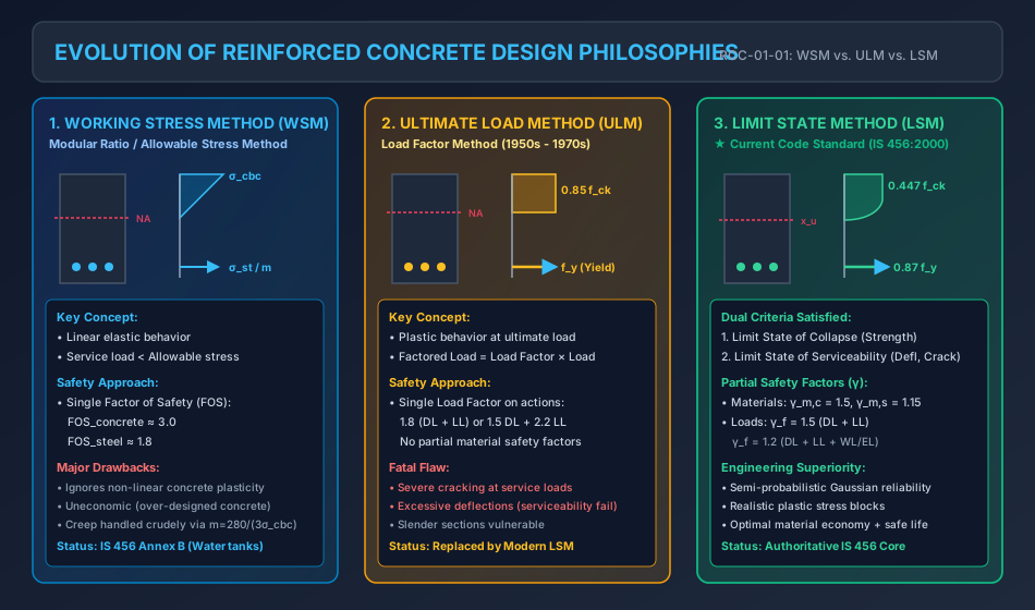
Over the past century, three distinct design philosophies have evolved for proportioning reinforced concrete members:
- The Working Stress Method (WSM): Elastic, modular-ratio-based allowable stress approach.
- The Ultimate Load Method (ULM): Plastic, load-factor-based ultimate collapse approach.
- The Limit State Method (LSM): Comprehensive, semi-probabilistic dual-criterion approach.
   1900 - 1950s: Working Stress Method (WSM) [Linear Elastic, Single FOS, Unrealistic Concrete Model]
        |
        +---> 1950s - 1970s: Ultimate Load Method (ULM) [Plastic at Collapse, Severe Cracking/Deflections]
        |
        +---> 1970s - Present: Limit State Method (LSM) [Dual Limit States: Collapse + Serviceability, Partial Factors]
2. The Working Stress Method (WSM) — Elastic / Modular Ratio Theory
The Working Stress Method (also known as Allowable Stress Design or Modular Ratio Theory) was the earliest rational method of concrete design. It is based on linear elastic theory and Hooke's law ().
2.1 Fundamental Assumptions (IS 456:2000 Annex B, Clause B-1.3)
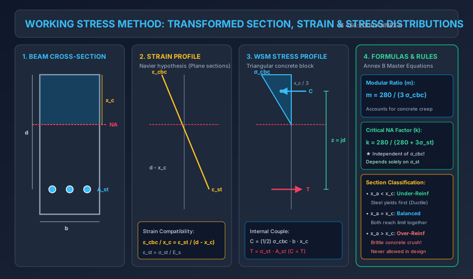
- Navier's Hypothesis: At any cross-section, plane sections before bending remain plane after bending across the entire depth. The strain distribution is strictly linear.
- Hooke's Law Holds: Both steel and concrete are assumed to behave as perfectly linear elastic materials up to their allowable working stresses.
- Tensile Concrete Neglected: All tensile stresses are resisted entirely by the tensile reinforcement. The tensile strength of concrete is ignored in flexural design.
- Perfect Bond: No relative slip occurs between concrete and surrounding steel bars ( at the reinforcement level).
- Modular Ratio (): The modular ratio is assumed constant and defined per IS 456:2000 Annex B as: where is the permissible compressive stress in concrete in bending ().
2.2 The Modular Ratio & The Long-Term Creep Phenomenon
The theoretical (short-term) modular ratio is defined strictly by the ratio of moduli of elasticity:
However, concrete undergoes significant time-dependent deformation under sustained loading (Creep). Creep increases concrete compressive strain by a factor of to , causing an internal redistribution that relieves concrete stress and increases the stress carried by the reinforcement.
To account partially for creep and non-linear plasticity in a simplified linear framework, IS 456:2000 specifies the effective / long-term modular ratio:
Engineering Significance: Notice that is inversely proportional to . For lower grade concrete (e.g., M15, ), . For higher grade concrete (e.g., M25, ), . This reflects the fact that lower grade concretes undergo significantly higher creep.
2.3 The Equivalent Transformed Section
Because steel has an elastic modulus times higher than concrete, an area of steel can carry times as much force as an equivalent area of concrete under the same strain:
Hence, the cracked composite cross-section is mathematically replaced by an Equivalent Transformed Concrete Section:
- Compression zone: Real concrete of width and depth .
- Tension zone: Effective concrete area equal to placed at effective depth .
3. Derivation of WSM Section Parameters & Neutral Axis Formulations
3.1 Critical (Balanced) Neutral Axis Depth ()
In a balanced section, the extreme outer compressive fiber of concrete reaches its permissible stress simultaneously as the tension steel reaches its permissible stress .
From the linear strain diagram (Navier hypothesis):
Since stresses are proportional to strains ( and ):
Let be the neutral axis depth factor:
Substitute the IS 456 definition :
[!IMPORTANT] Fundamental Examination Property: The critical neutral axis factor in WSM is completely independent of concrete grade ( or )! It depends solely on the permissible tensile stress in steel ():
- For Mild Steel (Fe 250, ):
- For Medium Tensile (Fe 415, ):
- For High Tensile (Fe 500, ):
3.2 Lever Arm () and Lever Arm Factor ()
Because the compressive stress distribution is triangular, the resultant compressive force acts at the centroid of the triangle, at a distance from the extreme compression fiber:
where is the lever arm factor.
3.3 Moment of Resistance Factor ()
- Resultant compressive force in concrete:
- Resultant tensile force in steel:
- Balanced Moment of Resistance (): where is the moment resisting factor.
3.4 Balanced Steel Reinforcement Percentage ()
Equating :
4. Section Classification in the Working Stress Method
In any given beam of dimensions with provided steel area , the actual depth of the neutral axis () is found by equating the first moment of area of the compression zone to that of the tension zone about the neutral axis:
Solving this quadratic equation yields . Comparing with the critical neutral axis depth yields three cases:
| Case | Condition | Physical State | First Material to Reach Limit | Failure Mode | Permissible Moment Capacity () |
|---|---|---|---|---|---|
| Under-Reinforced | Steel reaches first; | Ductile (Warning through wide cracks & deflection) | |||
| Balanced | Both reach and simultaneously | Simultaneous | |||
| Over-Reinforced | Concrete reaches first; | Brittle (Sudden, catastrophic concrete crushing) |
[!CAUTION] Code Restriction: In structural design, over-reinforced sections are strictly forbidden by IS 456 because concrete crushes abruptly without ductile warning. If an existing section is over-reinforced, its capacity must be limited strictly to the concrete compressive resistance, or compression reinforcement must be added (doubly reinforced beam).
5. The Ultimate Load Method (ULM) & Its Inherent Shortcomings
Developed in the 1950s (primarily based on Charles Whitney's equivalent rectangular stress block in ACI 318-56), the Ultimate Load Method abandoned linear elasticity in favor of plastic collapse behavior at the ultimate state.
5.1 Characteristics of ULM
- Evaluates the collapse capacity using non-linear plastic stress distribution across concrete.
- Applies a unified Load Factor () to the service loads: Typical load factors: or .
- Does not utilize separate partial safety factors for materials.
5.2 Deficiencies That Led to the Abandonment of ULM
- Serviceability Neglect: Because ULM focuses entirely on ultimate strength, slender, highly reinforced sections satisfied strength requirements but suffered severe cracking and excessive deflections under daily working loads.
- Arbitrary Safety Separation: A uniform load factor fails to distinguish between well-controlled dead loads (low uncertainty) and highly variable live or environmental loads (high uncertainty).
- Durability Failure: Large crack widths under service loads accelerated steel corrosion and concrete carbonation, leading to premature structural deterioration.
6. The Limit State Method (LSM) per IS 456:2000
The Limit State Method is a rational, semi-probabilistic design framework that bridges the gap between safety at ultimate collapse and performance during daily service.
6.1 Definition of a Limit State
A Limit State is a condition or boundary beyond which a structure becomes unfit for its intended purpose, failing to satisfy its design requirements.
IS 456:2000 classifies all limit states into two fundamental categories:
                          LIMIT STATES (IS 456:2000)
                                      |
         +----------------------------+----------------------------+
         |                                                         |
         v                                                         v
   LIMIT STATES OF COLLAPSE                                LIMIT STATES OF SERVICEABILITY
   (Ultimate Strength / Life Safety)                       (Daily Performance / Occupant Comfort)
   - Limit State of Collapse in Flexure                    - Limit State of Deflection
   - Limit State of Collapse in Compression (Columns)      - Limit State of Cracking
   - Limit State of Collapse in Shear                      - Limit State of Vibration
   - Limit State of Collapse in Torsion                    - Limit State of Durability & Fire
   - Limit State of Collapse in Bond & Anchorage
6.2 Partial Safety Factors for Materials ()
To account for variations in material strength, dimensions, and construction workmanship, the design strength is obtained by dividing characteristic strength by :
Per IS 456:2000 Clause 36.4.2:
- Concrete:
(Higher factor because concrete is manufactured under field conditions, subject to water-cement ratio variations, compaction, and curing differences). - Steel:
(Lower factor because reinforcing steel is industrially manufactured under strict factory quality control).
6.3 Partial Safety Factors for Loads ()
Per IS 456:2000 Table 18, factored design loads are obtained by multiplying characteristic loads by partial load factors :
| Load Combination | Limit State of Collapse () | Limit State of Serviceability () |
|---|---|---|
| Dead Load + Imposed Load (DL + IL) | ||
| Dead Load + Wind/Seismic (DL + WL/EL) | (or for stability) | |
| Dead + Imposed + Wind/Seismic (DL + IL + WL/EL) |
7. Comparative Architectural Summary: WSM vs. ULM vs. LSM
| Feature / Criterion | Working Stress Method (WSM) | Ultimate Load Method (ULM) | Limit State Method (LSM) |
|---|---|---|---|
| Core Philosophy | Deterministic / Elastic | Plastic Collapse | Semi-probabilistic / Dual Limit States |
| Stress Distribution | Linear triangular | Rectangular (Whitney) | Parabolic-Rectangular (IS 456) |
| Safety Factors | Single FOS on stresses ( for concrete, for steel) | Load Factor () on loads | Separate partial factors: (materials) and (loads) |
| Material Plasticity | Completely ignored | Fully mobilized at ultimate | Fully mobilized at collapse limit state |
| Serviceability Guarantee | Implicitly assumed (often uneconomic) | Violated (frequent excessive cracks/deflection) | Explicitly verified (deflection & crack width checks) |
| Section Economy | Heavy, over-sized concrete sections | Excessively thin, slender sections | Optimal, balanced, and highly economic |
| Long-Term Effects | Addressed crudely via | Neglected | Explicitly accounted for via creep & shrinkage factors |
| Current Code Status | Annex B of IS 456 (Special structures: liquid retaining) | Obsolete | Primary Design Method (IS 456, ACI 318, Eurocode 2) |
8. Worked Numerical Examples
Problem 1: WSM Balanced Section & Section Factors (M20 & Fe 415)
Statement: A singly reinforced rectangular beam has breadth and effective depth . The materials are grade M20 concrete () and grade Fe 415 steel (). Using the Working Stress Method per IS 456:2000 Annex B:
- Determine the modular ratio .
- Calculate the neutral axis depth factor , lever arm factor , and moment factor .
- Compute the balanced moment of resistance and the required balanced steel area .
- Find the balanced percentage of steel ().
Solution:
Step 1: Modular Ratio () Per IS 456:2000 Annex B, Clause B-1.3:
Step 2: Section Factors ()
- Neutral Axis Depth Factor ():
- Critical Neutral Axis Depth:
- Lever Arm Factor ():
- Lever Arm ():
- Moment Resisting Factor ():
Step 3: Balanced Moment of Resistance () and Steel Area ()
- Moment of Resistance:
- Required Balanced Steel Area ():
Step 4: Balanced Steel Percentage ()
Problem 2: WSM Analysis of an Under-Reinforced Section
Statement: A rectangular reinforced concrete beam has width and effective depth . The tension reinforcement consists of 3 bars of diameter. Permissible stresses are (M20) and (Mild Steel Fe 250).
- Determine the actual neutral axis depth () and compare it with the critical neutral axis depth ().
- Classify the section.
- Calculate the actual maximum compressive stress in concrete () when steel reaches its permissible limit.
- Calculate the moment of resistance ().
Solution:
Step 1: Section Properties and Critical Neutral Axis ()
- Steel area: .
- Modular ratio: .
- Critical neutral axis depth factor:
- Critical Neutral Axis Depth:
Step 2: Actual Neutral Axis Depth () Equating the first moments of area of the transformed section about the neutral axis:
Dividing by :
Solving using the quadratic formula:
Step 3: Section Classification & Concrete Stress
- Comparison: .
- Classification: The section is UNDER-REINFORCED.
- Steel reaches its allowable stress first.
- The actual extreme fiber concrete compressive stress () is: (Since , concrete operates comfortably within its safe elastic limit).
Step 4: Moment of Resistance () Governed by steel tension:
Problem 3: Quantitative Economic Comparison (WSM vs. LSM)
Statement: A beam cross-section with and is proportioned using M20 concrete () and Fe 415 steel ().
- From Problem 1, recall the WSM balanced capacity: with .
- Compute the balanced limiting moment of resistance under the Limit State Method () per IS 456:2000.
- Compute the required limiting steel area in LSM ().
- Convert to an equivalent working service moment () and evaluate the economy ratio .
Solution:
Step 1: Limiting Neutral Axis Depth in LSM (IS 456 Clause 38.1) For Fe 415 steel:
Step 2: Limiting Moment of Resistance ()
Step 3: Limiting Steel Area in LSM ()
Step 4: Comparison & Economic Assessment
- Equivalent service load moment in LSM (using dead + live load factor ):
- Ratio of Service Moment Capacity (LSM / WSM):
- Conclusion: For the same concrete dimensions (), the Limit State Method permits more than double () the working moment compared to WSM. WSM's artificial triangular stress block severely underestimates the plastic reserve strength of concrete, demanding excessively large cross-sections.
9. Common Misconceptions & Exam Pitfalls
[!CAUTION]
- Modular Ratio Formula Trap: Never use for WSM calculations unless explicitly instructed. IS 456 Annex B mandatorily specifies , which embeds the long-term creep effect.
- Neutral Axis Factor Independence: In objective exams, candidates often erroneously calculate by re-deriving with and . Remember: in , concrete grade cancels out completely! is identical for M15, M20, M25, and M50!
- Failure Mechanism in Over-Reinforced Beams: An over-reinforced beam in WSM crushes in concrete with zero warning. Never calculate its moment as , as steel stress never reaches .
- Partial Safety Factors: Do not confuse with FOS. In LSM, accounts for material variability (), while accounts for load variability ( for DL+LL). In WSM, a single lumped FOS ( on concrete, on steel) is used.
10. Comparative Summary & Master Formula Sheet
| Parameter / Constant | Formula / Value in WSM (Annex B) | Formula / Value in LSM (Clause 38) |
|---|---|---|
| Concrete Compressive Stress | Linear triangular: | Parabolic-Rectangular: |
| Modular Ratio () | Not applicable (Strain compatibility used) | |
| Neutral Axis Factor | ||
| Lever Arm Factor | ||
| Material Safety Factor | Concrete: ; Steel: | Concrete: ; Steel: |
| Balanced Steel Ratio |
11. Practice Questions & Competitive Examination Problems
Multiple Choice & Objective Questions
-
[GATE CE] In the Working Stress Method of design, the modular ratio is given by . This expression takes into account:
- (A) Only short-term elastic effects
- (B) Partially the effect of long-term creep
- (C) The effect of shrinkage only
- (D) The variation of steel yield strength
Answer: (B) Partially accounts for long-term creep of concrete.
-
[ESE CE] If is the permissible compressive stress in bending for concrete and is the permissible tensile stress in steel, the critical neutral axis depth factor depends upon:
- (A) Both and
- (B) only
- (C) only
- (D) Modulus of elasticity of concrete only
Answer: (C) In , cancels out; it depends only on .
-
[SSC JE] In the Limit State Method, the partial safety factor for concrete () is higher than that for steel () because:
- (A) Concrete is weaker in tension
- (B) Concrete has higher density
- (C) Concrete quality control in the field has greater uncertainty than factory-produced steel
- (D) Steel undergoes strain hardening
Answer: (C) Field quality control variability of concrete.
-
[State AE] In a singly reinforced beam, if the actual neutral axis depth is less than the critical neutral axis depth , the section is termed:
- (A) Balanced section
- (B) Over-reinforced section
- (C) Under-reinforced section
- (D) Critical section
Answer: (C) Under-reinforced section.
12. References & Code Standards
- IS 456:2000: Plain and Reinforced Concrete — Code of Practice (Fourth Revision), Bureau of Indian Standards, New Delhi.
- Clause 18: Design Concepts
- Clause 35 & 36: Limit State Method Principles & Safety Factors
- Annex B: Working Stress Method
- IS 3370 (Part 2): 2009: Code of Practice for Concrete Structures for the Storage of Liquids.
- SP 16:1980: Design Aids for Reinforced Concrete to IS 456:1978, BIS, New Delhi.
- Pillai, S. U., & Menon, D. (2021). Reinforced Concrete Design. Tata McGraw-Hill.
- Park, R., & Paulay, T. (1975). Reinforced Concrete Structures. John Wiley & Sons.