Characteristic Strengths, Characteristic Loads & Partial Safety Factors (IS 456:2000)
In this chapter (3 topics)
On this page
- 1. Introduction & Conceptual Foundations
- 2. Statistical Basis of Characteristic Values (Gaussian / Normal Distribution)
- 2.1 The Gaussian Probability Density Function
- 2.2 Derivation of the 1.645 Fractile Factor
- 3. Characteristic Strength of Materials (fk)
- 3.1 Characteristic Compressive Strength of Concrete (fck)
- 3.2 Standard Deviation Values per IS 456:2000 (Table 8)
- 3.3 Characteristic Yield / Proof Strength of Steel (fy)
- 4. Characteristic Loads (Fk)
- 4.1 Definition (IS 456:2000 Clause 36.2)
- 4.2 Standard Code References for Loads in India
- 5. Partial Safety Factors for Materials (γm)
- 5.1 Code Values (IS 456:2000 Clause 36.4.2)
- 5.2 Technical Justification: Why is γc (1.50) > γs (1.15)?
- 5.3 The In-Situ Concrete Characteristic Strength Factor (0.67)
- 5.4 Design Strength of Reinforcing Steel
- 6. Partial Safety Factors for Loads (γf) & Critical Load Combinations
- 6.1 Codified Values of γf per IS 456:2000 Table 18
- 6.2 Key Critical Observations on Table 18
- 7. Probabilistic Reliability & Structural Safety Concepts
- 7.1 The Fundamental Limit State Function
- 7.2 The Hasofer-Lind Reliability Index (β)
- 8. Worked Numerical Examples
- Problem 1: Concrete Compressive Test Evaluation & Design Parameters
- Problem 2: Critical Load Combination Envelope for a Multi-Story Column
- Problem 3: Probabilistic Reliability Index (β) & Structural Failure Probability
- 9. Common Misconceptions & Exam Pitfalls
- 10. Comparative Summary & Master Formula Sheet
- Master Mathematical Equations
- Code Partial Safety Factors Summary
- 11. Practice Questions & Competitive Examination Problems
- Question 1 (GATE CE — 1 Mark)
- Question 2 (UPSC ESE — Objective)
- Question 3 (SSC JE — Technical)
- Question 4 (State AE — Analytical)
- Question 5 (GATE CE — 2 Marks)
- Question 6 (UPSC ESE — Conventional)
- 12. References & Code Standards
1. Introduction & Conceptual Foundations
In structural engineering, neither material strengths nor external loads are deterministic single-value quantities. If one hundred standard concrete cubes are cast from identical ingredients and tested under identical laboratory protocols, their crushing strengths vary across a measurable dispersion. Similarly, the actual live loads, wind pressures, and earthquake accelerations sustained by a structure over a 50-year service life are stochastic (random) variables.
Early design philosophies tackled uncertainty through crude blanket measures:
- Working Stress Method (WSM): Applied an empirical Factor of Safety ( for concrete, for steel) solely to material yield/ultimate strength while treating applied loads as absolute, deterministic working values.
- Ultimate Load Method (ULM): Applied an arbitrary overall Load Factor ( to ) to service loads while treating material strengths at plastic collapse deterministically.
Both methods failed to decouple the distinct uncertainties arising from material quality control on the one hand, and load fluctuations on the other.
The Limit State Method (LSM), codified in IS 456:2000, adopts a semi-probabilistic approach (Level 1 Reliability). It formally separates uncertainties into:
- Characteristic Values (): Statistically defined cutoff thresholds with specified acceptance probabilities.
- Partial Safety Factors for Materials (): Accounting for manufacturing tolerances, in-situ casting defects, dimension reductions, and deterioration.
- Partial Safety Factors for Loads (): Accounting for load estimation errors, simultaneous occurrence probabilities, and unforeseen stress redistributions.
+----------------------------------------------------------------------------------------------------+
|                               THE SEMI-PROBABILISTIC DESIGN FRAMEWORK                              |
+----------------------------------------------------------------------------------------------------+
|                                                                                                    |
|   MATERIAL STRENGTH                                                      APPLIED LOADS             |
|   Mean Strength (fm)                                                     Mean Load (Fm)            |
|          |                                                                      |                  |
|          v  [Statistical Dispersion: -1.645 s]                                  v  [+1.645 s_L]    |
|   Characteristic Strength (fk)                                           Characteristic Load (Fk)  |
|          |                                                                      |                  |
|          v  [Divide by gamma_m]                                                 v  [Multiply by    |
|   Design Strength (fd = fk / gamma_m)                                              gamma_f]        |
|          |                                                                      |                  |
|          +---------------------------> DESIGN CHECK <---------------------------+                  |
|                                       Sd <= Rd                                                     |
|                        (Design Action Effect <= Design Resistance)                                 |
+----------------------------------------------------------------------------------------------------+
2. Statistical Basis of Characteristic Values (Gaussian / Normal Distribution)
Extensive empirical testing confirms that the compressive strength of concrete cubes and the yield strength of reinforcing steel closely follow a Gaussian (Normal) Probability Distribution.
2.1 The Gaussian Probability Density Function
For a continuous random variable representing material strength with mean (or ) and standard deviation (or ):
The standardized normal variable is dimensionless:
The cumulative probability is the area under the probability density curve:
   Relative Frequency f(x)
             ^
             |                             Mean fm
             |                                |
             |                               :*:
             |                             *  :  *
             |                           *    :    *
             |                         *      :      *
             |                       *        :        *
             |                     *          :          *
             |                   *            :            *
             |      5% Tail    *              :              *
             |      Area     *                :                *
             |       |     *                  :                  *
             +-------v---*--------------------+--------------------*-----> Strength x
                        ^                     ^
                        |                     |
                     fk = fm - 1.645 s        fm
                     (Characteristic)       (Mean)
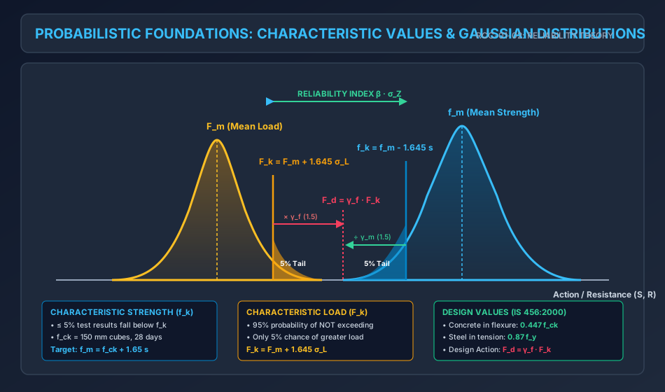
2.2 Derivation of the Fractile Factor
IS 456:2000 defines characteristic strength such that not more than 5 percent of the test results are expected to fall below it:
Using the standard normal cumulative distribution:
Looking up standard Gaussian probability tables:
- For ,
- For ,
Interpolating linearly:
In Indian standard practice and literature, this factor is written as (or precisely ):
Key Distinction for Competitive Exams:
- A 5% one-tailed cutoff requires .
- A 5% two-tailed cutoff (2.5% in each tail, i.e., 95% confidence interval) requires .
Because structural safety concerns only the lower tail (under-strength), IS 456 adopts the one-tailed .
3. Characteristic Strength of Materials ()
3.1 Characteristic Compressive Strength of Concrete ()
Per IS 456:2000 Clause 6.1.1:
Characteristic compressive strength () is defined as the strength of cubes at 28 days of curing, conducted in accordance with IS 516, below which not more than 5 percent of the test results are expected to fall:
Where:
- is the mean compressive strength of cube specimens ().
- is the sample standard deviation ().
- Concrete grade designation: An M25 concrete denotes a nominal mix or design mix having a characteristic 28-day cube compressive strength ().
3.2 Standard Deviation Values per IS 456:2000 (Table 8)
When conducting preliminary mix designs without site test data, IS 456:2000 Clause 9.2.4.2 mandates minimum assumed standard deviations:
| Concrete Grade Classification | Grade of Concrete | Assumed Standard Deviation () |
|---|---|---|
| Ordinary Concrete | M10, M15 | |
| Standard Concrete | M20, M25 | |
| Standard / High Strength | M30, M35, M40, M45, M50, M55, M60 |
Application to Mix Design (Target Mean Strength):
To guarantee that at least of field batches meet or exceed the specified , concrete mixes must be designed for a Target Mean Compressive Strength ():For example, for M25 concrete with good site control ():
3.3 Characteristic Yield / Proof Strength of Steel ()
Per IS 456:2000 Clause 5.6 & IS 1786:
- Mild Steel (Fe 250): Possesses a definite, well-defined yield plateau. The characteristic strength is taken as the guaranteed minimum yield stress ().
- High Yield Strength Deformed (HYSD / TMT) Bars (Fe 415, Fe 500, Fe 550D, Fe 600): Cold-worked or thermo-mechanically treated bars do not exhibit a distinct yield plateau. The characteristic strength is defined by the Proof Stress (), which corresponds to a permanent non-proportional strain of ().
4. Characteristic Loads ()
4.1 Definition (IS 456:2000 Clause 36.2)
Characteristic Load () is defined as that value of load which has an agreed percent probability of not being exceeded during the design working life of the structure.
Mathematically, for a normally distributed load variable with mean load and load standard deviation :
   Relative Frequency f(F)
             ^
             |                             Mean Load Fm
             |                                  |
             |                                 :*:
             |                               *  :  *
             |                             *    :    *
             |                           *      :      *
             |                         *        :        *
             |                       *          :          *
             |                     *            :            *
             |                   *              :              *
             |                 *                :                *  Upper 5% Tail
             |               *                  :                  *  (Overload)
             +-------------*--------------------+--------------------*-----> Load F
                                                ^                    ^
                                                |                    |
                                                Fm                   Fk = Fm + 1.645 s_L
                                              (Mean)           (Characteristic)
Notice the crucial directional difference:
- Material strength is safety-critical on the lower tail .
- Applied load is safety-critical on the upper tail .
4.2 Standard Code References for Loads in India
In practice, full statistical data for every individual building site is unavailable. Therefore, characteristic loads are prescribed directly as standard design loads in the Indian Standard load codes:
- Dead Loads (DL): Unit weights of building materials per IS 875 (Part 1): 1987. (e.g., Plain Concrete , Reinforced Concrete , Brick Masonry , Structural Steel ).
- Imposed / Live Loads (IL / LL): Occupancy loads per IS 875 (Part 2): 1987. (e.g., Residential floors , Corridors/Stairs , Office floors ).
- Wind Loads (WL): Dynamic wind pressures per IS 875 (Part 3): 2015 based on basic wind speed with a 50-year mean return period ( factors).
- Snow Loads (SL): Snow accumulation per IS 875 (Part 4): 1987.
- Earthquake / Seismic Loads (EL): Design lateral seismic forces per IS 1893 (Part 1): 2016 using seismic zone factor , importance factor , response reduction factor , and spectral acceleration coefficient .
5. Partial Safety Factors for Materials ()
To establish the Design Strength () of a material, its characteristic strength is divided by a Partial Safety Factor for Materials ():
5.1 Code Values (IS 456:2000 Clause 36.4.2)
| Material | Limit State of Collapse | Limit State of Serviceability |
|---|---|---|
| Concrete () | ||
| Steel Reinforcement () |
5.2 Technical Justification: Why is ?
This is one of the most frequent conceptual questions in competitive examinations (GATE, UPSC ESE, State AE/JE). The higher safety factor for concrete () compared to steel () is governed by three fundamental factors:
-
Manufacturing Environment & Quality Control:
- Reinforcing steel is manufactured under strictly controlled metallurgical conditions in automated industrial rolling mills. Chemical composition, thermal quenching, and rolling tolerances are monitored with high-precision instrumentation, resulting in minimal statistical variance (coefficient of variation ).
- Structural concrete is batch-mixed, transported, poured, compacted, and cured in-situ under open-air site conditions. Workmanship, water-cement ratio variations, aggregate grading fluctuations, incomplete compaction, and erratic field curing introduce significant dispersion ().
-
Dimensional & Cross-Sectional Tolerances:
- Concrete members (beams, slabs, columns) are shaped using temporary wooden or steel formwork. Misalignment, shuttering deflection, or cover block displacements directly reduce the effective depth . Because bending capacity scales with , a small dimensional error causes a severe capacity drop. Steel bars, by contrast, maintain precise cross-sectional diameters.
-
Material Homogeneity & Degradation:
- Concrete is a heterogeneous, multiphase composite susceptible to micro-cracking, shrinkage, creep, and environmental chemical ingress (carbonation, chloride attack). Steel is an isotropic, homogeneous material with predictable ductile yielding.
5.3 The In-Situ Concrete Characteristic Strength Factor ()
In flexural design, the design compressive strength of concrete is formulated as:
Derivation of the Factor:
Why is multiplied by before dividing by ?
- Size / Specimen Effect (): Standard test specimens are small cubes. In an actual full-scale structural member, volumetric size effects, heterogeneous aggregate packing, and internal bleeding reduce the compressive capacity relative to a small cube. Tests show that in-situ concrete reaches only about of standard cube strength:
- Sustained Load Duration Effect ( to ): Cube crushing tests are conducted under rapid loading (loading rate , failure in 2 to 3 minutes). Under sustained long-term dead and service loads over decades, static fatigue / creep rupture lowers the ultimate strength by an additional to :
Therefore, represents the true characteristic strength of concrete inside the actual structure. Dividing this in-situ characteristic strength by the material partial safety factor yields:
5.4 Design Strength of Reinforcing Steel
For reinforcing steel, cross-sectional area and yield strength are directly verified in the factory. No specimen-to-structure reduction factor is necessary:
6. Partial Safety Factors for Loads () & Critical Load Combinations
To establish the Design Load (), the characteristic load is multiplied by a Partial Safety Factor for Loads ():
The factor accounts for:
- Possibility of unfavorable deviations of loads from characteristic values.
- Unforeseen stress redistribution due to settlement, cracking, or thermal variations.
- Inaccuracies in structural analysis models (e.g., idealized knife-edge supports, 2D planar frames).
- Limit state consequences (consequence of collapse vs serviceability impairment).
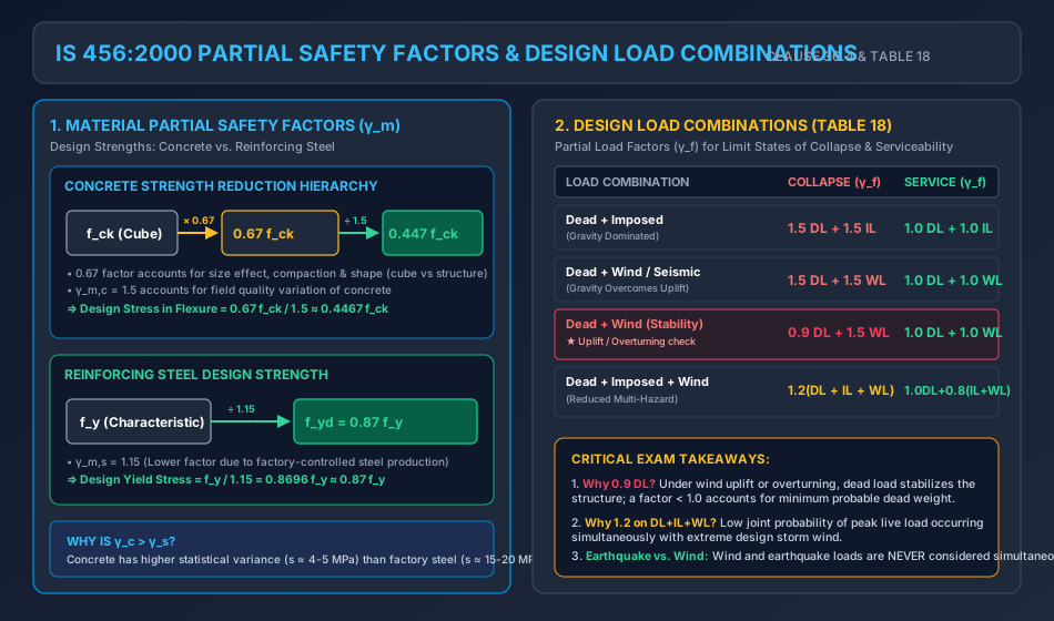
6.1 Codified Values of per IS 456:2000 Table 18
| Load Combination | Limit State of Collapse | Limit State of Serviceability |
|---|---|---|
| 1. Dead Load + Imposed Load | ||
| 2. Dead Load + Wind/Earthquake Load | ||
| - Normal condition (Overturning / Stresses) | ||
| - Adverse / Reversal condition (Uplift / Stability) | — | |
| 3. Dead Load + Imposed Load + Wind/Earthquake Load |
6.2 Key Critical Observations on Table 18
- The Stability Combination:
- Under lateral wind or seismic forces, dead load provides stabilizing gravity moments against overturning, foundation uplift, and tension anchorage failure.
- When dead load acts to counteract overturning or uplift, applying would be dangerously un-conservative. IS 456 mandates reducing the dead load factor to to account for the possibility of lighter construction finishes or missing partitions.
- The Simultaneous Three-Load Combination ( Factor):
- When dead load, full live load, and peak design wind/seismic load act simultaneously, the joint probability of all three reaching their extreme characteristic peaks concurrently is exceedingly small.
- Hence, is reduced from to for collapse.
- Mutual Exclusivity of Wind (WL) and Earthquake (EL):
- Per IS 456 Clause 36.4.1 and IS 1893:2016, wind load and earthquake load need never be considered simultaneously. Design checks consider whichever action governs the member.
- Serviceability Reduction for Transient Loads:
- For serviceability under , the factor for transient loads is reduced to ().
7. Probabilistic Reliability & Structural Safety Concepts
To understand the theoretical foundation beneath semi-probabilistic Level 1 codes, modern structural engineering evaluates safety through the Reliability Index ().
7.1 The Fundamental Limit State Function
Let:
- = Structural Resistance / Capacity (random variable with mean and standard deviation ).
- = Applied Solicitations / Load Effect (random variable with mean and standard deviation ).
The Safety Margin / Performance Function () is defined as:
A structure violates its limit state (fails) when:
   Probability Density
             ^
             |                 Load S                       Resistance R
             |               [mu_S, sigma_S]               [mu_R, sigma_R]
             |                    :                             :
             |                   / \                           / \
             |                  /   \                         /   \
             |                 /     \   INTERFERENCE        /     \
             |                /       \    FAILURE          /       \
             |               /         \    ZONE           /         \
             |              /           \  (Z < 0)        /           \
             |             /             \  ||||         /             \
             +------------+---------------+--||+--------+---------------+-----> Magnitude (S, R)
                                            ^^
                                            Overlap = Failure Probability Pf
7.2 The Hasofer-Lind Reliability Index ()
If and are independent normally distributed random variables, is also normally distributed:
The Reliability Index () measures the distance between the mean safety margin and the failure threshold () in units of standard deviations:
The probability of structural failure () is given by the standard normal distribution:
| Reliability Index | Failure Probability | Target Structural Application (ISO 2394) |
|---|---|---|
| ( in ) | Temporary / Agricultural structures | |
| ( in ) | Serviceability limit states | |
| ( in ) | Typical civil buildings (50-year life) | |
| ( in ) | Primary bridge girders / Public infrastructure | |
| ( in ) | Critical post-disaster facilities, dams |
Calibration of IS 456:
The partial safety factors are mathematically calibrated so that standard RCC flexural and axial members achieve an operational target reliability index to ( to ).
8. Worked Numerical Examples
Problem 1: Concrete Compressive Test Evaluation & Design Parameters
Problem Statement:
A concrete batching plant produces M25 grade concrete for a major highway viaduct. Thirty standard cube specimens cured for 28 days yield a mean compressive strength with a sample standard deviation .
- Determine the characteristic compressive strength () achieved on site and verify whether the concrete meets the M25 specification per IS 456:2000.
- Calculate the design compressive strength () of the concrete in the structure at the limit state of collapse.
- Compute the target mean compressive strength () required for future mix design if the site control maintains .
Step-by-Step Solution:
Part 1: Field Characteristic Compressive Strength ()
Per IS 456:2000 Clause 6.1.1:
Substitute the measured site values:
Since , the concrete satisfies the M25 specification.
Part 2: Design Compressive Strength ()
The design compressive strength incorporates the size/duration effect () and the material partial safety factor ():
Part 3: Target Mean Strength for Mix Design ()
Per IS 456 Clause 9.2.4.2 and IS 10262:
Given specified and standard deviation (from Table 8):
Problem 2: Critical Load Combination Envelope for a Multi-Story Column
Problem Statement:
An interior perimeter column in a multi-story building sustains the following service load effects at its base cross-section:
- Dead Load (DL): Axial compressive load , Bending moment .
- Imposed Live Load (LL): Axial compressive load , Bending moment .
- Wind Load (WL): Lateral wind blowing perpendicular to the frame creates an overturning uplift tension force of on this column (i.e., ) and a lateral bending moment .
Determine the governing factored design axial force () and factored design bending moment () for all four codified load combinations under the Limit State of Collapse (IS 456:2000 Table 18).
Step-by-Step Solution:
Combination 1: Gravity Only ()
Combination 2: Dead Load + Wind Load ()
Combination 3: Reversal / Minimum Dead Load + Wind ()
(Note: If had evaluated to a negative value, the column would experience net tensile uplift, requiring full tensile splices and anchor bolts).
Combination 4: Combined Gravity + Wind ()
Comparison and Design Envelope:
- Maximum Axial Compression: Governed by Combination 1 ().
- Maximum Bending Moment: Governed by Combination 2 ().
- Critical Minimum Axial Load with High Moment (Tension Governed): Evaluated under Combination 3 ().
Problem 3: Probabilistic Reliability Index () & Structural Failure Probability
Problem Statement:
A reinforced concrete transfer girder has a normally distributed flexural moment resistance with a mean and standard deviation (). The applied maximum service bending moment is also normally distributed with a mean and standard deviation ().
- Compute the mean () and standard deviation () of the safety margin .
- Calculate the Hasofer-Lind reliability index ().
- Determine the theoretical probability of flexural failure ().
Step-by-Step Solution:
Part 1: Statistical Parameters of Safety Margin
Because and are statistically independent normal variables:
Part 2: Hasofer-Lind Reliability Index ()
Part 3: Probability of Failure ()
The probability of failure is:
Evaluating standard Gaussian probability integrals:
This corresponds to a risk of approximately failure in every identical girders over their design working life.
9. Common Misconceptions & Exam Pitfalls
[!WARNING] Pitfall 1: Confusing the Factor with a Factor of Safety
Students often mistakenly write that is a safety factor. In fact, is a specimen-to-structure physical conversion factor that accounts for specimen size effects () and long-term sustained loading effects (). The actual safety factor is , applied in the denominator:
[!WARNING] Pitfall 2: Neglecting the Combination in Stability
In retaining walls, cantilever bridge piers, and water tanks, students frequently check only . When dead load acts to stabilize against overturning, uplift, or base sliding, the dead load must be reduced using . Using overestimates the stabilizing resisting moment and leads to unsafe designs.
[!CAUTION] Pitfall 3: Assuming for all Loads in Serviceability
While uses factors of , the three-load serviceability combination () uses:Forgetting the reduction factor for transient loads is a frequent error in GATE serviceability deflection checks.
[!IMPORTANT] Pitfall 4: Misinterpreting vs
In statistics, corresponds to a two-tailed confidence interval ( in each tail). In IS 456, characteristic strength is defined by a one-tailed lower exclusion limit, which strictly requires (commonly rounded to ).
10. Comparative Summary & Master Formula Sheet
Master Mathematical Equations
| Quantity | Formula | Governing IS 456 Clause |
|---|---|---|
| Characteristic Strength | Clause 6.1.1 | |
| Target Mean Strength (Mix Design) | Clause 9.2.4.2 | |
| Characteristic Load | Clause 36.2 | |
| Concrete Design Strength (Collapse) | Clause 38.1 | |
| Steel Design Strength (Collapse) | Clause 38.1 | |
| Reliability Index () | Probabilistic Safety Theory | |
| Probability of Failure () | Hasofer-Lind Formulation |
Code Partial Safety Factors Summary
+-----------------------------------------------------------------------------------------------+
|                                    IS 456:2000 SAFETY FACTORS                                 |
+----------------------------------------------------+--------------------+---------------------+
| Condition / Element                                | Limit State of     | Limit State of      |
|                                                    | Collapse           | Serviceability      |
+----------------------------------------------------+--------------------+---------------------+
| Concrete (gamma_c)                                 | 1.50               | 1.00                |
| Reinforcing Steel (gamma_s)                        | 1.15               | 1.00                |
| DL + LL                                            | 1.5 DL + 1.5 LL    | 1.0 DL + 1.0 LL     |
| DL + WL/EL (Overturning / Stresses)                | 1.5 DL + 1.5 WL    | 1.0 DL + 1.0 WL     |
| DL + WL/EL (Uplift / Stability)                    | 0.9 DL + 1.5 WL    | --                  |
| DL + LL + WL/EL                                    | 1.2(DL + LL + WL)  | 1.0DL + 0.8LL+0.8WL |
+----------------------------------------------------+--------------------+---------------------+
11. Practice Questions & Competitive Examination Problems
Question 1 (GATE CE — 1 Mark)
As per IS 456:2000, the characteristic compressive strength of concrete is defined as the strength below which not more than:
- (A) 10% of test results are expected to fall
- (B) 5% of test results are expected to fall
- (C) 2.5% of test results are expected to fall
- (D) 1% of test results are expected to fall
Answer: (B)
Explanation: IS 456 Clause 6.1.1 specifies the 5% lower fractile ().
Question 2 (UPSC ESE — Objective)
The design compressive stress of concrete in limit state flexural design is taken as . The factor incorporated into this value represents:
- (A) Partial safety factor for concrete
- (B) Specimen size effect and sustained load effect
- (C) Long-term creep factor of concrete
- (D) Ratio of cylindrical to cubical compressive strength
Answer: (B)
Explanation: The ratio converts 28-day cube test strength to the real-life member compressive strength under sustained load ().
Question 3 (SSC JE — Technical)
For concrete mix design of M30 grade concrete, if standard deviation is not established by field trials, the assumed standard deviation per IS 456:2000 Table 8 is:
- (A)
- (B)
- (C)
- (D)
Answer: (C)
Explanation: Table 8 specifies for M10/M15, for M20/M25, and for M30 to M60.
Question 4 (State AE — Analytical)
A building is subject to a characteristic Dead Load of , characteristic Imposed Load of , and characteristic Earthquake Load of . The factored design load under the Limit State of Collapse considering all three loads simultaneously is:
- (A)
- (B)
- (C)
- (D)
Answer: (B)
Explanation: Factored load .
Question 5 (GATE CE — 2 Marks)
In a cantilever retaining wall, the characteristic dead load stabilizing moment against overturning is , and the characteristic overturning overturning moment caused by lateral earth and water pressure is . The design margin of safety against overturning under the Limit State of Collapse (using the critical stability load factor) is:
- (A)
- (B)
- (C)
- (D)
Answer: (A)
Explanation: For stability against overturning, for dead load and for lateral load. Design stabilizing moment . Design overturning moment . Margin of safety .
Question 6 (UPSC ESE — Conventional)
Explain why the partial safety factor for concrete () is higher than that for steel reinforcement ().
Answer Summary: Concrete is cast in-situ with significant variability in mixing, compaction, and curing (), and is prone to formwork dimensional errors and micro-cracking. Steel is industrially manufactured under strict quality control () with precise geometric tolerances.
12. References & Code Standards
- IS 456:2000 (Reaffirmed 2021): Plain and Reinforced Concrete — Code of Practice, Section 5 (Clause 36: Limit State Design, Clause 38: Limit State of Collapse — Flexure, Table 18: Partial Safety Factors).
- IS 875 (Parts 1–5): Code of Practice for Design Loads (Other than Earthquake) for Buildings and Structures.
- IS 1893 (Part 1): 2016: Criteria for Earthquake Resistant Design of Structures.
- IS 10262:2019: Concrete Mix Proportioning — Guidelines.
- ISO 2394:2015: General Principles on Reliability for Structures.
- Pillai, S. U., & Menon, D. (2021): Reinforced Concrete Design, 4th Edition, McGraw-Hill Education.
- Varghese, P. C. (2009): Limit State Design of Reinforced Concrete, 2nd Edition, PHI Learning.