Influence Lines for Determinate Beams and Girders
In this chapter (4 topics)
On this page
- 1. Introduction & Physical Motivation
- 1.1 Critical Comparison: SFD/BMD vs. ILD
- 2. First-Principles Mathematical Derivation of Elementary ILDs
- 2.1 ILD for Support Reactions (RA and RB)
- 2.2 ILD for Shear Force at Section C (VC)
- 2.3 ILD for Bending Moment at Section C (MC)
- 3. The Müller-Breslau Principle for Determinate Beams
- Application to Statically Determinate Structures:
- 4. Engineering Diagrams & Visual Explanations
- 4.1 Elementary ILDs on Simply Supported Beams
- 4.2 Overhangs, Internal Hinges & Indirect Floor Girders
- 5. ILDs for Overhangs, Compound Beams & Internal Hinges
- 5.1 Beams with Overhangs
- 5.2 Compound Beams with Internal Hinges (Gerber Beams)
- 6. Indirect Loading in Bridge Girders (Floor Beams, Stringers & Panels)
- Fundamental Theorem of Indirect Loading:
- 7. Quantitative Evaluation of Moving Loads on ILD
- 7.1 Single Concentrated Load (P)
- 7.2 System of Concentrated Loads (Σ Pi)
- 7.3 Uniformly Distributed Load of Uniform Intensity (w)
- 8. Solved Numerical Examples
- Example 1: Simply Supported Beam with Overhang Under Moving Point Load and Finite UDL
- Example 2: Compound Beam with Internal Hinge (Gerber Beam)
- Example 3: Bridge Floor Girder with Indirect Panel Loading
- 9. Practical Engineering Applications & Bridge Standards
- 9.1 IRC:6-2017 Bridge Design Vehicles
- 9.2 Impact Allowance (Dynamic Load Amplification)
- 10. Common Misconceptions & Exam Traps
- 1. Confusing ILD with SFD / BMD
- 2. Neglecting the Discontinuity Jump in Shear ILD
- 3. Load Positioning for Maximum Sagging Moment under Finite UDL
- 4. Floor Girder Panel Shear Jump Misconception
- 11. Practice Problems
- Problem 1 (GATE CE Standard)
- Problem 2 (UPSC ESE Conventional Standard)
- 12. Quick Revision Formula Summary
1. Introduction & Physical Motivation
In structural design, loads are classified into two broad categories:
- Dead Loads (Stationary Loads): Permanent, non-moving loads such as the self-weight of beams, slabs, ballast, and permanent utilities.
- Live Loads (Moving Loads): Variable, transient loads whose position changes over time, including highway trucks, railway locomotives, gantry crane trolleys, and pedestrian crowds.
To analyze a structure subjected to stationary dead loads, we construct standard Shear Force Diagrams (SFD) and Bending Moment Diagrams (BMD). However, when loads move across a bridge or crane girder, the internal forces at every cross-section vary continuously with the position of the moving vehicle.
To determine:
- Where a moving vehicular load must be placed to produce the worst-case (maximum) bending moment or shear force at a critical cross-section, and
- What the exact magnitude of that worst-case internal force is,
we utilize an indispensable graphical and analytical tool: the Influence Line Diagram (ILD).
Fundamental Concept:
┌────────────────────────────────────────────────────────────────────────┐
│ An Influence Line Diagram (ILD) for a specific structural response     │
│ function (reaction, shear force, or bending moment at a chosen section)│
│ is a graph showing the variation of that response function as a single │
│ downward unit point load (1 kN) rolls across the entire span.          │
└────────────────────────────────────────────────────────────────────────┘
1.1 Critical Comparison: SFD/BMD vs. ILD
| Comparative Parameter | Shear Force / Bending Moment Diagram (SFD / BMD) | Influence Line Diagram (ILD) |
|---|---|---|
| Loading Condition | Fixed, stationary loads at designated, permanent locations. | A single unit load () moving across the span. |
| Abscissa (-axis) | Represents the position of any cross-section along the beam. | Represents the position of the rolling unit load. |
| Ordinate (-axis) | Value of internal shear () or moment () at that cross-section. | Value of reaction, shear, or moment at one fixed section . |
| Scope of Coverage | Covers all sections of the beam under one load case. | Covers all possible load locations for one fixed section. |
| Dimensional Units | Shear: , Moment: . | Reaction: , Shear: , Moment: . |
2. First-Principles Mathematical Derivation of Elementary ILDs
Consider a simply supported beam of span resting on a pin support at () and a roller support at (). A unit vertical downward point load () moves from left to right, located at a variable distance from support .
           1 kN (Unit Moving Load)
             ↓
  A ─────────┴───────────────────────────────── B
 [▲]  x                                        [▲]
  │◄───────────────────── L ──────────────────►│
2.1 ILD for Support Reactions ( and )
Using global equations of static equilibrium:
-
Left Support Reaction ():
Taking moments about right support :- When the unit load is at (): .
- When the unit load is at midspan (): .
- When the unit load is at (): .
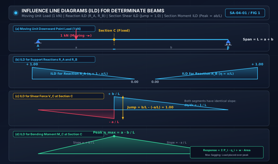
- The ILD for is a straight line sloping downward from at to at .
-
Right Support Reaction ():
Taking moments about left support :- When the unit load is at (): .
- When the unit load is at (): .
- The ILD for is a straight line sloping upward from at to at .
Notice that at any position :
2.2 ILD for Shear Force at Section ()
Let section be located at a fixed distance from left support , and distance from right support .
By sign convention, transverse shear force is positive if the left segment shears upward relative to the right segment:
  A                    Section C                     B
 [▲]───────────────────────│────────────────────────[▲]
  │◄───────── a ──────────►│◄────────── b ──────────►│
Case 1: Unit Load to the Left of Section ()
Considering all forces to the right of section :
- At (load at support ): .
- As the load approaches section from the left ():
- The ordinate is negative (downward triangular lobe).
Case 2: Unit Load to the Right of Section ()
Considering all forces to the left of section :
- As the load is placed immediately to the right of section ():
- When the load reaches support (): .
- The ordinate is positive (upward triangular lobe).
Key Properties of Shear Force ILD:
- Vertical Step Discontinuity (Jump):
At section , the shear force undergoes an instantaneous jump: The jump magnitude is always exactly equal to the magnitude of the unit moving load ()! - Parallel Slopes:
The slope of the line to the left of is .
The slope of the line to the right of is .
Both segments are strictly parallel straight lines with slope .
2.3 ILD for Bending Moment at Section ()
By sign convention, bending moment is positive (sagging) if it produces tension in the bottom fibers and compression in the top fibers.
Case 1: Unit Load to the Left of Section ()
Considering the right-hand segment of the beam:
- At : .
- At (unit load directly at section ):
- The slope is .
Case 2: Unit Load to the Right of Section ()
Considering the left-hand segment of the beam:
- At : .
- At : .
- The slope is .
Key Properties of Bending Moment ILD:
- Triangular Shape with Positive Peak:
The ILD is a triangle with base , zero ordinates at both supports, and a maximum positive peak ordinate directly below section : - Dimensional Unit:
Notice that the ordinate has dimensions of (meters), because multiplying this ordinate by a point load directly gives bending moment in .
3. The Müller-Breslau Principle for Determinate Beams
In 1886, the German civil engineer Heinrich Müller-Breslau formulated a profound kinematic principle connecting virtual work with influence lines:
Müller-Breslau Principle:
┌────────────────────────────────────────────────────────────────────────┐
│ The Influence Line Diagram for any internal or external force function │
│ (reaction, shear, or moment) represents, to some scale, the deflected  │
│ shape of the structure obtained by removing the restraint corresponding│
│ to that function and introducing a unit displacement in its direction. │
└────────────────────────────────────────────────────────────────────────┘
Application to Statically Determinate Structures:
In a statically determinate structure, removing any single restraint (reaction constraint, shear capacity, or rotational continuity) removes all static redundancy, instantly converting the structure into a kinematic mechanism consisting of rigid-body segments:
- Because the structural segments remain rigid and do not bend, the resulting influence lines for all determinate structures consist strictly of straight lines!
- For Shear : Cut the beam at , insert a frictionless vertical slide guide, and translate the two cut faces vertically relative to each other by a unit distance (). The displaced rigid profile is the exact ILD for !
- For Moment : Cut the beam at , insert an internal frictionless pin hinge, and apply opposing unit rotations (). The tent-like rigid deflected shape is the exact ILD for !
4. Engineering Diagrams & Visual Explanations
4.1 Elementary ILDs on Simply Supported Beams
The diagram below provides a unified visual comparison of the four canonical influence lines on a simply supported beam: Left Reaction , Right Reaction , Shear Force at Section , and Bending Moment at Section .
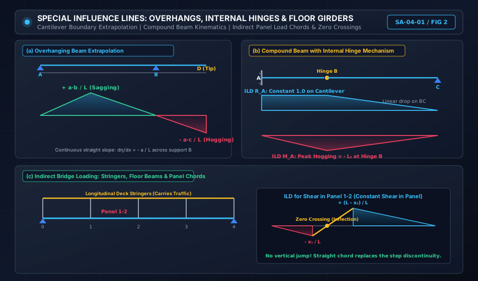
4.2 Overhangs, Internal Hinges & Indirect Floor Girders
Special structural configurations introduce distinctive kinematic behaviors:
- Overhanging Beams: Linear extrapolation past the supports produces negative hogging moment lobes and reaction reversals.
- Compound Beams with Hinges: Cantilevered segments transfer loads unidirectionally across internal hinges.
- Indirect Floor Girder Loading: Floor beams distribute rolling loads onto main girders exclusively at discrete panel points, replacing step discontinuities with continuous straight chords.
5. ILDs for Overhangs, Compound Beams & Internal Hinges
5.1 Beams with Overhangs
Consider a beam supported at and of span , with an overhanging cantilever of length extending to the right of support to tip (Total length ):
- Reaction :
The line continues linearly past : When the load is on the overhang, support experiences an upward holding-down force (negative reaction) to prevent overturning! - Reaction :
The line continues linearly past : The reaction exceeds because support acts as a fulcrum. - Bending Moment at Span Section ():
The line from the peak passes through zero at support () and extends linearly onto the overhang: A load on the overhang causes hogging (negative) moment at all interior span sections!
5.2 Compound Beams with Internal Hinges (Gerber Beams)
A Gerber beam utilizes internal hinges to make multi-span systems statically determinate ().
Consider a compound beam fixed at wall , with an internal hinge at (), and a simple roller support at ():
- Segment is supported by a roller at and the internal hinge at . It behaves like a simply supported beam of span .
- Segment is a cantilever fixed at , supporting the hinge at its free tip.
Kinematic Rules for Hinged Compound Beams:
- Loads on Cantilever :
Loads placed between and are carried entirely by the fixed support . Zero load is transferred to segment All response functions in () are identically zero for loads on ! - Loads on Supported Span :
A load on is shared between support () and the hinge ().
The reaction acts as a concentrated downward point load on the tip of cantilever , inducing reactions and fixed-end moment .
6. Indirect Loading in Bridge Girders (Floor Beams, Stringers & Panels)
In real bridges, vehicle wheels do not roll directly on top of the main trusses or plate girders. Instead, the bridge floor system consists of:
- Stringers: Longitudinal beams spanning parallel to traffic.
- Cross-Girders (Floor Beams): Transverse beams located at discrete intervals (panel points) supported by the main girders.
Bridge Deck Hierarchy:
Wheel Load (1 kN) ──► Longitudinal Stringer ──► Floor Beams at Panel Points ──► Main Girder
When a rolling unit load is located at distance between panel point and panel point (panel width ):
- The stringer transfers reactions to the two adjacent floor beams:
- The main girder receives loads only at panel points and .
Fundamental Theorem of Indirect Loading:
The influence line for any internal stress function (shear force or bending moment) in a girder subjected to indirect loading consists of straight lines connecting the exact influence line ordinates calculated at the discrete panel points!
Implications for Shear Force in Panel :
In direct loading, the shear ILD has a vertical jump of at section . In indirect floor-beam loading:
- The shear force is uniform across the entire panel.
- The vertical step discontinuity is replaced by a straight sloping chord connecting the ordinate at panel point () to the ordinate at panel point ().
- This chord crosses the baseline, creating a zero-crossing point (inflection) inside the panel:
7. Quantitative Evaluation of Moving Loads on ILD
Once the ILD for a response function (reaction, shear, or moment) is drawn, the actual response produced by any combination of real loads is evaluated using two fundamental integration theorems:
7.1 Single Concentrated Load ()
If a concentrated load is placed at position where the ILD ordinate is :
- To maximize positive response: Place directly at the maximum positive peak ordinate .
- To maximize negative response: Place directly at the maximum negative peak ordinate .
7.2 System of Concentrated Loads ()
For a train of rolling point loads located at positions corresponding to ordinates :
7.3 Uniformly Distributed Load of Uniform Intensity ()
Consider a differential load element at position . The response produced is .
Integrating along the loaded length from to :
Optimization Criteria for Distributed Loads:
- Maximum Positive Response ():
- If the UDL is longer than the span: Place the UDL to cover all positive lobes of the ILD.
- If the UDL has a finite length : Place the load over the region of the positive lobe having the highest average ordinate. For a triangular ILD, the peak must divide the load length in the same ratio as the peak divides the span: The end ordinates under the head and tail of the distributed load must be strictly equal!
- Maximum Negative Response ():
Place the UDL to cover all negative lobes of the ILD.
8. Solved Numerical Examples
Example 1: Simply Supported Beam with Overhang Under Moving Point Load and Finite UDL
Problem Statement:
A beam of total length is supported on a simple pin at () and a roller at (), with a cantilever overhang extending to tip ().
Section is chosen in the interior span at from support .
The beam is traversed by two concurrent live loads moving from left to right:
- A single concentrated point load .
- A uniformly distributed load of finite length with intensity .
Determine:
- Maximum positive and negative shear force at section ( and ).
- Maximum positive (sagging) and negative (hogging) bending moment at section ( and ).
   A                   Section C                     B       Overhang D
  [▲]──────────────────────│────────────────────────[▲]───────────
   x = 0                x = 4 m                   x = 10 m   x = 12 m
   │◄──────── 4 m ────────►│◄──────── 6 m ──────────►│◄── 2 m ──►│
Solution:
Step 1: Construct the ILD for Shear Force at Section ()
- Span .
- At (support ): .
- Immediately left of (): .
- Immediately right of (): .
- At (support ): .
- Extrapolation onto overhang ():
The line passes through and with slope .
At : .
Step 2: Maximum Positive Shear Force at ()
The positive lobe of the ILD lies entirely between and .
- Point Load : Place immediately to the right of ():
- Finite UDL ():
Place the load starting at and ending at to capture the highest positive ordinates.
Ordinate at : .
Area under ILD: - Total Maximum Positive Shear:
Step 3: Maximum Negative Shear Force at ()
Negative lobes exist on (maximum ordinate ) and on (maximum ordinate ).
- Point Load : Place immediately to the left of ():
- Finite UDL ():
Place the UDL on the segment where ordinates are largest negative.
At : . At : .
Area of trapezoid: - Total Maximum Negative Shear:
Step 4: Construct the ILD for Bending Moment at Section ()
- Span peak at ():
- Zero at supports () and ().
- Overhang Tip (): Extrapolating straight line through and :
Step 5: Maximum Sagging Moment at ()
- Point Load : Place directly at section ():
- Finite UDL ():
The load must straddle the peak at () such that the peak divides the load in the ratio : Check end ordinates:- At : .
- At : ! (Identical, confirming maximum area!).
Total Area under the UDL:
- Total Maximum Sagging Moment:
Step 6: Maximum Hogging Moment at ()
The negative lobe exists exclusively on the cantilever overhang between and .
- Point Load : Place at the cantilever tip ():
- Finite UDL ():
The overhang length is , so the UDL can only occupy on the negative lobe: - Total Maximum Hogging Moment:
Example 2: Compound Beam with Internal Hinge (Gerber Beam)
Problem Statement:
A compound beam is fixed at wall (), contains an internal hinge at (), and rests on a simple roller support at ().
A critical evaluation section is located at (the exact midpoint of supported span ).
Construct the ILD equations and key coordinates for:
- Vertical reaction and fixed-end moment at wall .
- Vertical reaction at roller support .
- Shear force and bending moment at section .
Solution:
Step 1: Structural Kinematics
- Span has length . It is supported by roller and the hinge .
- Span is a cantilever of length , fixed at .
Step 2: ILD for Reaction
- When unit load is on cantilever ():
No force is transferred across hinge to span . - When unit load is on span ():
Span is simply supported. Taking moments about hinge :- At (hinge ): .
- At (support ): .
Step 3: ILD for Reaction
- When unit load is on cantilever ():
The entire load is carried directly by wall : . - When unit load is on span ():
The vertical reaction at hinge is .
This downward reaction at transfers directly to wall :- At : .
- At : .
Step 4: ILD for Fixed-End Moment
- When unit load is on cantilever ():
Clockwise/anticlockwise: Downward load creates hogging moment : At : . At (hinge ): . - When unit load is on span ():
The downward force on cantilever tip is .
The moment at wall is : At : . At : .
Step 5: ILD for Shear and Moment at Midspan ()
- For loads on (): Zero internal force in .
- For loads on (): Span acts as a simple span of with at its center ():
- Shear :
Just left of (): .
Just right of (): .
Jump at . - Moment :
Peak at :
- Shear :
Example 3: Bridge Floor Girder with Indirect Panel Loading
Problem Statement:
A plate girder bridge has an overall span of supported simply at its ends () and ().
The bridge floor system divides the main girder into equal panels of length via floor beams located at panel points (), (), (), (), and ().
- Derive and plot the ILD for shear force in Panel (between and ).
- Locate the zero-crossing point (inflection point) within the panel.
- Determine the maximum positive and negative shear force produced in Panel by a rolling uniformly distributed dead and live load of intensity of unlimited length.
Solution:
Step 1: ILD Ordinates at Panel Points for Panel Shear
In indirect loading, the shear force is identical across any section in the panel.
- When unit load is at panel point ():
The load is entirely to the left of the cut in Panel : - When unit load is at panel point ():
The load is entirely to the right of the cut in Panel : - Across Panel (from to ), the ILD is a straight continuous chord connecting to !
Step 2: Zero-Crossing (Inflection Point) Location
Using linear interpolation between and :
The shear in Panel changes from negative to positive when the wheel load passes !
Step 3: Maximum Shear Forces under Unlimited UDL ()
-
Maximum Positive Shear ():
Load must occupy the entire positive lobe, extending from to .- Area of triangle from to (base , height ):
- Area of triangle from to (base , height ):
- Total Positive Area .
-
Maximum Negative Shear ():
Load must occupy the entire negative lobe, extending from to .- Area of triangle from to (base , height ):
- Area of triangle from to (base , height ):
- Total Negative Area .
9. Practical Engineering Applications & Bridge Standards
9.1 IRC:6-2017 Bridge Design Vehicles
In Indian highway engineering (IRC:6-2017 Section 204), bridge decks and girders must be analyzed for moving standard vehicle trains:
- IRC Class 70R Tracked Vehicle: heavy military tracked tank ( ground contact).
- IRC Class 70R Wheeled Vehicle: 7-axle heavy transport bogie.
- IRC Class A Train Vehicle: 8-axle commercial truck train. Engineers calculate ILDs at intervals of across the bridge girder, and run algorithmically stepped axle configurations across the ILD to generate the maximum design bending moment envelope.
9.2 Impact Allowance (Dynamic Load Amplification)
Because rolling bridge vehicles bounce dynamically over road roughness, the static response calculated from the ILD must be amplified by an Impact Factor ():
For steel highway bridges under IRC Class A loading:
10. Common Misconceptions & Exam Traps
[!WARNING]
1. Confusing ILD with SFD / BMD
Exam Trap: Plotting the variation of shear along the length of the beam for a fixed point load at midspan and calling it an ILD.
Reality: An SFD evaluates all sections under fixed loads. An ILD evaluates one fixed section as a unit load moves across all positions!
[!WARNING]
2. Neglecting the Discontinuity Jump in Shear ILD
Exam Trap: Drawing the shear ILD as a continuous line through section .
Reality: The shear force ILD MUST have an instantaneous vertical step of exactly at section ().
[!WARNING]
3. Load Positioning for Maximum Sagging Moment under Finite UDL
Exam Trap: Placing the front of a finite UDL at the section peak to maximize moment.
Reality: To maximize moment under a finite UDL of length , the peak of the ILD must divide the load length in the same ratio that the section divides the span:Placing the load symmetrically or arbitrarily without equalizing end ordinates leads to significant under-design!
[!WARNING]
4. Floor Girder Panel Shear Jump Misconception
Exam Trap: Drawing a vertical jump in the ILD inside a bridge panel.
Reality: In indirect floor-beam systems, wheel loads reach the girder only through floor beams. There is NO vertical step inside the panel; the ILD is a smooth, continuous straight chord connecting the adjacent panel point ordinates!
11. Practice Problems
Problem 1 (GATE CE Standard)
A simply supported beam of span is traversed by a rolling uniformly distributed live load of intensity and length .
Determine the absolute maximum bending moment that can be produced at the quarter-span section ().
Answer:
Peak ordinate .
Load division ratio: (left of peak), (right of peak).
End ordinates: .
Area of trapezoid .
.
Problem 2 (UPSC ESE Conventional Standard)
A beam has a supported span and two equal overhanging cantilevers and (Total length ).
Construct the ILD for shear force and bending moment at midspan of . Determine the length and placement of a rolling UDL of intensity to produce:
- The maximum sagging bending moment at midspan.
- The maximum hogging bending moment at midspan.
Answer:
- For maximum sagging moment: Peak . Place UDL to cover span entirely ():
. - For maximum hogging moment: Overhang tip ordinates . Place UDL over both cantilevers and ( total length):
.