Principle of Virtual Work & Unit Load Method for Deflection of Trusses, Beams & Frames
In this chapter (3 topics)
On this page
- 1. Executive Summary & Engineering Significance
- 2. Theoretical Foundations of Virtual Work
- 2.1 The Two Duality Principles of Virtual Work
- 2.2 The Dummy Unit Load Theorem
- 3. Mathematical Formulations & General Equations
- 3.1 Pin-Jointed Plane and Space Trusses
- 3.2 Flexural Beams and Rigid Frames
- 3.3 Vereshchagin's Rule & Product Integrals
- 4. Graphical Displacement Analysis: The Williot-Mohr Method
- 4.1 Kinematic Stages of Truss Joint Motion
- 4.2 Construction Steps of the Williot Diagram
- 4.3 The Mohr Correction Diagram
- 5. Engineering Visualizations
- 5.1 Unit Load Method & Virtual Work Duality
- 5.2 Williot-Mohr Graphical Construction
- 6. Comparative Engineering Matrix
- 7. Solved Numerical Examples with Rigorous Proofs
- Example 1: Symmetrical Roof Truss under External Load, Temperature Change, and Fabrication Defect
- Example 2: Stepped Cantilever Beam under Combined UDL and Concentrated Tip Load
- Example 3: Deep Cantilever Beam — Flexural vs Shear Deflection Breakdown
- 8. Common Pitfalls, Exam Traps & Misconceptions
- 8.1 The "Factor of 1/2" Virtual Work Fallacy
- 8.2 The Algebraic Sign Rule for Temperature & Lack-of-Fit
- 8.3 The Non-Linearity Limit of Vereshchagin's Multiplication Rule
- 8.4 The Extensibility Oversight in Rigid Frame Sway Analysis
- 9. Codal Provisions & Real-World Engineering Context
- 9.1 IS 800:2007 Deflection Limits (Table 6)
- 9.2 Thermal Gradient Considerations in IS 456:2000 & IRC:24-2010
- 10. Previous Year Questions & Master Formula Sheet
- 10.1 Representative Competitive Exam Questions
- 10.2 Master Formula Sheet
1. Executive Summary & Engineering Significance
In structural engineering, the determination of displacements (deflections and slopes) is essential for:
- Serviceability Limit State Verification: Ensuring deflections under service loads remain within codal limits (such as or per IS 800:2007 and IS 456:2000) to prevent damage to architectural finishes, ponding of water, or excessive vibrations.
- Analysis of Statically Indeterminate Structures: Formulating compatibility equations in classical force methods (such as the Method of Consistent Deformations and the Method of Least Work).
While elementary geometric techniques (Double Integration, Macaulay's Method, and Moment-Area Theorems) excel for simple prismatic beams, they become unwieldy for pin-jointed trusses, non-prismatic members, combined flexure-shear-axial systems, and space structures.
The Principle of Virtual Work and its operational corollary, the Dummy Unit Load Method (often attributed to Maxwell, Mohr, and Vereshchagin), provides a universal, mathematically elegant, energy-based framework applicable to any linearly or non-linearly elastic structure. It seamlessly handles:
- Mechanical nodal and distributed loads
- Thermal expansion and thermal gradients ()
- Fabrication errors and lack-of-fit ()
- Support settlements and rotations ()
2. Theoretical Foundations of Virtual Work
2.1 The Two Duality Principles of Virtual Work
Virtual work theorems arise from variational principles in continuum mechanics and exist in two complementary forms:
| Characteristic | Principle of Virtual Displacements (Real Forces) | Principle of Virtual Forces / Unit Load Method (Virtual Forces) |
|---|---|---|
| Primary System | Real, equilibrium force field or | Real, compatible deformation field or |
| Imposed System | Imaginary, kinematically admissible virtual displacement | Imaginary, statically admissible virtual force field or |
| Governing Equation | ||
| Primary Structural Application | Displacement formulation; Stiffness Matrix derivation; Upper-bound plastic collapse limit analysis. | Force formulation; Unit Load Method for deflections; Flexibility Matrix derivation. |
2.2 The Dummy Unit Load Theorem
To calculate the specific displacement at point in direction due to actual loads, temperature, or fabrication errors:
- Apply an imaginary, dimensionless virtual unit load () at point in direction . If a rotation is desired, apply a dummy virtual unit couple ( or dimensionless unity).
- The virtual unit load creates an internal virtual stress/force field (, member forces , virtual bending moments ).
- The real external loads create an actual strain/displacement field (, real member elongations , real curvatures ).
- By the Principle of Virtual Forces, external virtual work equals internal virtual work:
Key Distinction: There is no factor of in the virtual work equation. The real deformations occur throughout the entire existence of the constant virtual force, so work done is force displacement, not the area under a triangle.
3. Mathematical Formulations & General Equations
3.1 Pin-Jointed Plane and Space Trusses
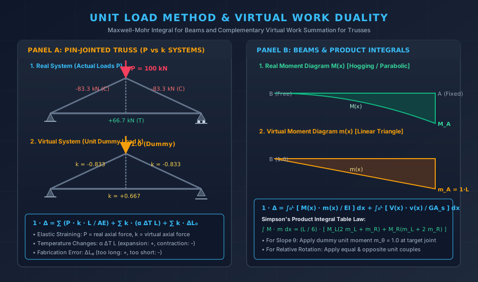
For a pin-jointed truss where members carry only axial forces, the total deformation of each member consists of:
- Elastic straining due to real forces :
- Thermal expansion/contraction due to uniform temperature change :
- Fabrication error / initial lack-of-fit: (positive if fabricated too long, negative if fabricated too short)
The internal virtual work becomes the sum over all members:
Where:
- : Desired nodal displacement component.
- : Real internal axial force in member under actual external loads.
- : Virtual internal axial force in member under a virtual unit load applied at the node and in the direction of .
- : Length, cross-sectional area, Young's modulus, and coefficient of thermal expansion of member .
Specialized Truss Displacement Queries:
- Relative Displacement between two distant joints and : Apply two equal and opposite unit collinear loads of at joints and .
- Angular Rotation of a Truss Line / Member: Apply a unit couple consisting of two parallel forces of magnitude separated by distance at the two ends.
3.2 Flexural Beams and Rigid Frames
In flexural systems, internal deformations arise from bending moment , shear force , axial thrust , and torsional moment . By integrating across the length of all members:
Where:
- : Real internal force resultants due to actual applied loading.
- : Virtual internal force resultants caused by the dummy unit load ().
- : Form factor for shear ( for rectangles, for solid circles, for I-beam webs where ).
Primary Contributions Hierarchy:
For slender beams and civil engineering frames with slenderness ratio :
- Flexural Strain Energy: Accounts for to of total deflection.
- Shear Energy: Accounts for and is typically neglected unless members are deep beams ().
- Axial Energy: Negligible in unbraced flexural beams; significant in arches, cables, and tall sway frames.
Slope and Rotation Formulation:
To compute the slope at any section :
where is the bending moment diagram caused by an applied dummy unit couple at point .
Temperature Gradient in Beams:
If a beam experiences a linear temperature differential between top fiber () and bottom fiber ():
3.3 Vereshchagin's Rule & Product Integrals
Computing analytically for multi-span frames can be time-consuming. Vereshchagin's Rule converts the definite integral into a simple geometric multiplication:
Vereshchagin's Condition: If at least one of the two moment diagrams () is strictly linear over the integration interval , the integral equals the area of the real moment diagram multiplied by the ordinate of the linear diagram measured directly under the centroid of the real diagram:
Real Moment M(x):    [   Area A_M   ]  ---> Centroid at distance x_c
                            |
Virtual Moment m(x): _______v_______  ---> Ordinate at x_c is m_c
                     \      |      /
                      \     m_c   /
Canonical Product Integral Results (Simpson's Table):
| Shape 1: (Length ) | Shape 2: (Linear, Length ) | Integral Value |
|---|---|---|
| Rectangle (height ) | Rectangle (height ) | |
| Rectangle (height ) | Triangle (height at end) | |
| Triangle (height at left) | Triangle (height at left) | |
| Triangle (height at left) | Triangle (height at right) | |
| Parabola (UDL, apex ) | Rectangle (height ) | |
| Parabola (UDL, apex ) | Triangle (height at end) | |
| Trapezoid () | Trapezoid () |
4. Graphical Displacement Analysis: The Williot-Mohr Method
Before numerical computing, truss deflections were determined graphically using the Williot-Mohr diagram. It remains a fundamental tool for visualizing the kinematic deformation of framed systems.
4.1 Kinematic Stages of Truss Joint Motion
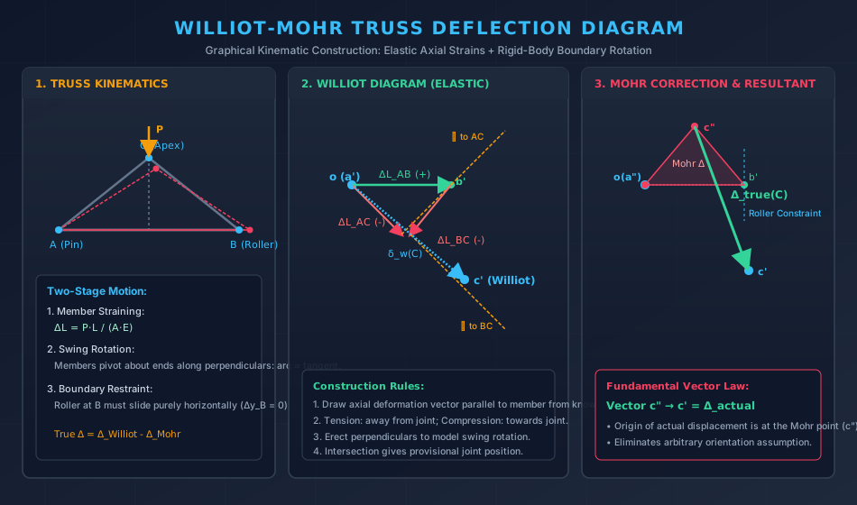
When a truss carries load, every pin joint undergoes motion through two stages:
- Primary Linear Translation (Elastic Elongation/Shortening): Every member changes length by . Joint displacement occurs along the member's initial axis.
- Secondary Rotational Translation (Swing Arc): Because connected members must stay pinned together, each member swings through a small angle about its opposite joint. For infinitesimal elastic deformations, the circular swing arc is accurately represented by a perpendicular tangent line.
4.2 Construction Steps of the Williot Diagram
- Pick an Arbitrary Fixed Joint and Reference Direction: Assume Joint is stationary and member does not rotate.
- Set Pole (Origin): Pole represents zero displacement ().
- Plot Member Axial Strain Vectors:
- Draw vector parallel to member with magnitude equal to . (Tension: draw in direction from to ; Compression: draw opposite).
- Erect Perpendiculars:
- At the tip of the axial deformation vectors, draw perpendicular lines representing the swing rotation.
- The intersection of these perpendiculars locates the provisional displaced joint position ().
- Repeat across all triangular panels.
4.3 The Mohr Correction Diagram
The raw Williot diagram assumes that an initial member has zero rotation. However, real boundary conditions dictate that:
- One support () is pinned (zero translation in and ).
- The second support () rests on a roller, constrained to move strictly along the guide surface (e.g., purely horizontally, meaning ).
The arbitrary orientation in the Williot diagram generally causes joint to exhibit an illegal transverse displacement. The Mohr Correction eliminates this error by rotating the entire truss as a rigid body about the pinned support :
- A Mohr diagram is constructed, which is geometrically similar to the original truss layout, rotated by .
- The scale of the Mohr triangle is calibrated so that the displacement vector at the roller support restores the roller onto its true guide plane ().
- True Absolute Joint Displacement:
where is the point on the Mohr correction diagram and is the point on the Williot diagram.
5. Engineering Visualizations
5.1 Unit Load Method & Virtual Work Duality
5.2 Williot-Mohr Graphical Construction
6. Comparative Engineering Matrix
| Analysis Method | Primary Application | Basis of Method | Boundary Conditions Handled | Computational Effort |
|---|---|---|---|---|
| Unit Load Method (Virtual Work) | Trusses, non-prismatic beams, frames, combined effects | Work-Energy variational duality () | Universal (Loads, , , support slips) | Moderate; direct integration or table lookup |
| Castigliano's 2nd Theorem | Elastic indeterminate structures, single deflection points | Strain energy partial derivative () | Linear elastic materials only | Moderate; requires fictitious dummy loads if no real load exists |
| Moment-Area Theorems | Prismatic/stepped beams with continuous slope changes | Geometric integration of diagrams | Requires known slope/deflection reference points | Low for simple beams; complex for multi-story frames |
| Conjugate Beam Method | Beams with internal hinges and complex support types | Equivalence of shear/moment in fictitious conjugate beam | Beams only; supports transform into conjugate counterparts | Low to moderate for beams; not applicable to trusses |
| Williot-Mohr Diagram | Visual and graphic determination of all truss joints | Graphic kinematic vector synthesis + rigid-body rotation | Hinged and roller-supported trusses | High drafting effort; excellent pedagogical and diagnostic value |
7. Solved Numerical Examples with Rigorous Proofs
Example 1: Symmetrical Roof Truss under External Load, Temperature Change, and Fabrication Defect
Problem Statement:
A pin-jointed steel roof truss consists of three members: two rafters and of length , and a horizontal bottom tie of span . The apex is at a height of above horizontal tie . Joint is pinned, and joint is on a horizontal roller. All members have cross-sectional area and Young's modulus (). The coefficient of thermal expansion is .
The truss is simultaneously subjected to:
- A vertical downward load of applied at apex .
- A uniform temperature rise of in the bottom tie .
- Member was fabricated too short ().
Determine the total vertical deflection at apex .
                 B (Apex)
                 /\
                /  \
      L = 5 m  /    \  L = 5 m, h = 3 m
              /      \
             /________\
            A          C
                8 m
Solution:
Step 1: Geometry and Virtual Angles:
Step 2: Real Member Axial Forces (): Under vertical apex load :
- Support reactions by symmetry: , , .
- Joint equilibrium at :
- By symmetry:
Step 3: Virtual Member Axial Forces (): Apply a downward dummy unit load of at apex :
- Virtual reactions: , .
- Virtual member forces (proportional to real loads with factor ):
Step 4: Breakdown of Deflection Components:
-
Elastic Deflection under Applied Load ():
- Member :
- Member :
- Member :
-
Thermal Deflection due to Heating in Tie ():
-
Fabrication Error Deflection due to Short Rafter ():
Step 5: Total Vertical Apex Deflection:
Example 2: Stepped Cantilever Beam under Combined UDL and Concentrated Tip Load
Problem Statement:
A cantilever beam of length is fixed at support () and free at tip (). The beam is non-prismatic with stepped flexural rigidity:
- Segment (): Flexural rigidity
- Segment (): Flexural rigidity
The beam carries a uniformly distributed load of over the entire span, and a concentrated vertical load of at the free end . Given and (), calculate the vertical tip deflection at using the Unit Load Method.
Fixed A                       C                        Free B
  |===========================|--------------------------|
  |-------- 2 EI -------------|---------- EI ------------|  ↓ P = 30 kN
  |========= 3.0 m ===========|======== 3.0 m ===========|
   ↓↓↓↓↓↓↓↓↓↓↓↓↓↓↓↓↓↓↓↓↓↓↓↓↓↓↓↓↓↓↓↓↓↓↓↓↓↓↓↓↓↓↓↓↓↓↓↓↓↓↓↓↓↓ w = 20 kN/m
Solution:
Step 1: Coordinate System: Measure coordinate starting from free end towards fixed end ( at , at ).
Step 2: Real Bending Moment Function : At any distance from the free end:
Step 3: Virtual Bending Moment Function : Apply a downward virtual unit load of at free end :
The product is:
Step 4: Integration over the Two Segments:
-
Segment ( to , Rigidity ):
-
Segment ( to , Rigidity ):
- Evaluate at :
- Evaluate at :
Step 5: Total Tip Deflection:
Substituting :
Example 3: Deep Cantilever Beam — Flexural vs Shear Deflection Breakdown
Problem Statement:
A rectangular deep cantilever beam of breadth and overall depth is fixed at one end and carries a concentrated tip load . The material has and Shear Modulus . The shear form factor for a rectangular cross section is .
- For a span of (), calculate the flexural deflection , the shear deflection , the total tip deflection , and the percentage contribution of shear.
- If the span is reduced to (), recompute the shear contribution percentage.
- Calculate the tip rotation for the beam under a concentrated tip moment of .
Solution:
Section Properties:
- Area
- Second Moment of Area
- Flexural Rigidity
- Shear Rigidity
Step 1: Deflection Formulations:
- Real load: , .
- Virtual unit downward load at tip: , .
Step 2: Case 1 ():
Step 3: Case 2 (, Deep Beam):
Physical Conclusion: While shear deflection is only for , it jumps to for , proving why classical Euler-Bernoulli beam theory fails and Timoshenko beam theory is mandated for deep beams.
Step 4: Tip Rotation under ():
- Real moment: (constant hogging).
- Virtual unit moment at tip: (constant).
8. Common Pitfalls, Exam Traps & Misconceptions
8.1 The "Factor of 1/2" Virtual Work Fallacy
- Trap: Writing by analogy with real strain energy .
- Correction: The factor of applies only when a force increases linearly from to . In virtual work, the virtual load is applied prior to the real deformation and remains at full value throughout the deformation. Thus, work is strictly .
8.2 The Algebraic Sign Rule for Temperature & Lack-of-Fit
- Trap: Forgetting that virtual force can be negative.
- Rule:
If a member is fabricated short () and its virtual force is compression (), the product is (positive, meaning the joint deflects in the direction of the dummy unit load!). Always maintain rigorous signs:
- for Tension, for Compression.
- for Temperature Rise, for Temperature Fall.
- for Too Long, for Too Short.
8.3 The Non-Linearity Limit of Vereshchagin's Multiplication Rule
- Trap: Multiplying two non-linear diagrams using .
- Rule: Vereshchagin's theorem is valid only if at least one diagram is strictly linear over the interval. If both diagrams are non-linear (e.g., UDL on both real and virtual systems), Simpson's rule or direct integration must be used.
8.4 The Extensibility Oversight in Rigid Frame Sway Analysis
- Trap: Neglecting axial deformation in tall slender towers or portal frames with large horizontal spans.
- Rule: In low-rise rigid frames, axial deformations are minor compared to bending. However, for columns in tall structures, column shortening accumulates floor-by-floor and must be included via .
9. Codal Provisions & Real-World Engineering Context
9.1 IS 800:2007 Deflection Limits (Table 6)
To prevent architectural cracking, ponding, and elevator shaft misalignment, calculated elastic deflections must satisfy:
| Structural Element | Design Condition | Permissible Deflection Limit |
|---|---|---|
| Purlins & Girts | Elastic deflection under live/wind load | |
| Industrial Roof Trusses | Elastic deflection under live load | to |
| Floor Beams / Girders | Live load deflection (plastered ceiling) | to |
| Crane Gantry Girders | Manually operated crane | |
| Crane Gantry Girders | Electric overhead traveling (EOT) crane | to |
9.2 Thermal Gradient Considerations in IS 456:2000 & IRC:24-2010
In large concrete bridges and industrial roofs, top slabs exposed to direct solar radiation become significantly hotter than shaded bottom webs, creating thermal bowing moments:
The Unit Load Method is standard practice in bridge design software to compute long-term thermal deflections and joint displacements.
10. Previous Year Questions & Master Formula Sheet
10.1 Representative Competitive Exam Questions
Question 1 (GATE CE):
A pin-jointed truss has a member of length , area , and modulus . When a vertical load acts on the truss, the axial force in this member is . When a unit horizontal load is applied at joint , the axial force in this member is . If the member undergoes a temperature increase , its contribution to the horizontal deflection at joint is:
- (A)
- (B)
- (C)
- (D)
Answer: (C)
Explanation: By the Principle of Virtual Work, total horizontal displacement at is .
Question 2 (UPSC ESE):
In the Williot-Mohr diagram for a truss, the Mohr correction diagram is constructed primarily to:
- (A) Account for non-linear elastic behavior
- (B) Eliminate the shear deformation of the truss members
- (C) Correct for the arbitrary assumed rotation and satisfy actual boundary support conditions
- (D) Account for fabrication tolerances
Answer: (C)
Explanation: The Williot diagram assumes an arbitrary fixed direction for one member. The Mohr diagram represents a rigid body rotation about the pin support that enforces the true guide constraints at roller supports.
Question 3 (SSC JE):
For a cantilever beam of span and constant flexural rigidity subjected to a point load at its free end, the deflection at the free end computed using the unit load method is:
- (A)
- (B)
- (C)
- (D)
Answer: (B)
Explanation: .