SA-06-03 Chapter 06 · Matrix Methods of Structural Analysis

Matrix Analysis of 2D Frames & Grid Structures

In this chapter (4 topics)
On this page

1. Introduction & Executive Overview

Planar framed structures and orthogonal grid systems represent the overwhelming majority of real-world civil engineering infrastructure—from multi-story building frames, industrial bents, and bridge piers to floor slab grillages and bridge decks. While simple beam systems involve only transverse shear and flexure, 2D frames couple axial forces with flexure and shear, requiring coordinate transformations to resolve member orientations. Furthermore, grid structures (grillages) introduce out-of-plane flexure coupled with torsional resistance (GJGJ), expanding the computational formulation into three-dimensional behavior.

                          STRUCTURAL SYSTEMS CLASSIFICATION
   ┌──────────────────────────────┬──────────────────────────────┬──────────────────────────────┐
   │       2D PINNED TRUSS        │       2D RIGID FRAME         │      ORTHOGONAL GRID         │
   ├──────────────────────────────┼──────────────────────────────┼──────────────────────────────┤
   │ • 2 DOFs / Node: [u, v]      │ • 3 DOFs / Node: [u, v, θz]  │ • 3 DOFs / Node: [w, θx, θy] │
   │ • Axial Only (EA/L)          │ • Axial + Shear + Flexure    │ • Flexure + Torsion (GJ/L)   │
   │ • 4×4 Element Stiffness      │ • 6×6 Element Stiffness      │ • 6×6 Element Stiffness      │
   │ • Zero Member Moments        │ • Sway & Non-Sway Behavior   │ • Out-of-Plane Load (Pz)     │
   └──────────────────────────────┴──────────────────────────────┴──────────────────────────────┘

Key Engineering Objectives in This Topic:

  1. Formulate the Complete 6×66 \times 6 Frame Element Stiffness Matrix [kˉ][\bar{k}] in local coordinates, combining axial stiffness (EAL\frac{EA}{L}) and flexural stiffness (12EIL3,6EIL2,4EIL,2EIL\frac{12EI}{L^3}, \frac{6EI}{L^2}, \frac{4EI}{L}, \frac{2EI}{L}).
  2. Derive the 2D Planar Transformation Matrix [T][T] (6×66 \times 6) using direction cosines (λx,λy\lambda_x, \lambda_y) to rotate local member actions into the global frame.
  3. Analyze Sway vs. Non-Sway Portal Frames: Understand how the inextensibility assumption reduces degrees of freedom and master the global lateral shear equilibrium equation (∑H=0\sum H = 0).
  4. Formulate Grid Structures (Grillages): Establish the 3 DOFs per grid node (w,θx,θyw, \theta_x, \theta_y), formulate the 6×66 \times 6 grid element stiffness matrix coupling flexure (EIEI) and torsion (GJGJ), and analyze load sharing in orthogonal intersecting beams.

2. Fundamentals & Physical Mechanics

2.1 Degrees of Freedom in 2D Frames

A general 2D rigid joint in a plane frame can translate horizontally (uu), translate vertically (vv), and rotate in-plane (θ=θz\theta = \theta_z). Thus, each unconstrained joint has 3 degrees of freedom:

{d}joint=[uvθ]T\{d\}_{\text{joint}} = \begin{bmatrix} u & v & \theta \end{bmatrix}^T

For a frame with jj joints, rsr_s support restraints, and mrelm_{\text{rel}} internal moment releases (hinges):

Dk=3j−rs−mrel(considering axial deformation)D_k = 3j - r_s - m_{\text{rel}} \quad \text{(considering axial deformation)}
The Axial Inextensibility Assumption:

In most low-to-medium rise civil frames, axial stiffness (EAL\frac{EA}{L}) is orders of magnitude larger than flexural stiffness (12EIL3\frac{12EI}{L^3}):

EA/L12EI/L3=AL212I=L212rg2=λ212≫1\frac{EA/L}{12EI/L^3} = \frac{A L^2}{12 I} = \frac{L^2}{12 r_g^2} = \frac{\lambda^2}{12} \gg 1

For a typical column with slenderness λ=50\lambda = 50, the axial stiffness is over 200200 times stiffer than its lateral flexural stiffness. Consequently, assuming inextensible members (infinitely rigid axially):

  1. Columns do not change length   ⟹  \implies Joint vertical translations v=0v = 0.
  2. Beams do not change length   ⟹  \implies Joint horizontal translations across a floor level are equal (uB=uC=⋯=Δswayu_B = u_C = \dots = \Delta_{\text{sway}}).
  3. The degrees of freedom for a single-bay, single-story portal frame drop from 6 DOFs down to 3 DOFs ([Δ,θB,θC]T[\Delta, \theta_B, \theta_C]^T).

2.2 Degrees of Freedom in Grid Structures (Grillages)

A grid structure lies entirely in the XYXY plane, but external loads act perpendicular to the plane (in the ZZ-direction). Because deformation occurs strictly out-of-plane:

  1. In-plane translations ux,uyu_x, u_y and in-plane rotation θz\theta_z are zero.
  2. The active degrees of freedom at any grid joint are: {d}grid node=[wθxθy]T\{d\}_{\text{grid node}} = \begin{bmatrix} w & \theta_x & \theta_y \end{bmatrix}^T
    • ww: Vertical displacement along the ZZ-axis.
    • θx\theta_x: Rotation about the XX-axis (twisting torque for XX-parallel beams, bending moment for YY-parallel beams).
    • θy\theta_y: Rotation about the YY-axis (bending moment for XX-parallel beams, twisting torque for YY-parallel beams).

3. Mathematical Derivations & Theoretical Formulations

3.1 2D Frame Element Stiffness Matrix in Local Coordinates

Consider a prismatic member of length LL, cross-sectional area AA, moment of inertia II, and elastic modulus EE. The local displacement vector with 6 DOFs is:

{dˉ}=[uˉ1vˉ1θˉ1uˉ2vˉ2θˉ2]T\{\bar{d}\} = \begin{bmatrix} \bar{u}_1 & \bar{v}_1 & \bar{\theta}_1 & \bar{u}_2 & \bar{v}_2 & \bar{\theta}_2 \end{bmatrix}^T
       v̄1, θ̄1                                      v̄2, θ̄2
        ▲   ╭─╮                                     ▲   ╭─╮
        │   │ ↻                                     │   │ ↻
   ū1 ──●───┴───────────────────────────────────────●───┴──► ū2
       (1)                                         (2)
        └────────────────────── L ──────────────────┘

The corresponding internal force vector is:

{pˉ}=[Nˉ1Vˉ1Mˉ1Nˉ2Vˉ2Mˉ2]T\{\bar{p}\} = \begin{bmatrix} \bar{N}_1 & \bar{V}_1 & \bar{M}_1 & \bar{N}_2 & \bar{V}_2 & \bar{M}_2 \end{bmatrix}^T

Combining axial bar mechanics (Nˉ=±EALuˉ\bar{N} = \pm \frac{EA}{L}\bar{u}) with Euler-Bernoulli beam flexure (Vˉ=±12EIL3vˉ±6EIL2θˉ\bar{V} = \pm \frac{12EI}{L^3}\bar{v} \pm \frac{6EI}{L^2}\bar{\theta}, Mˉ=±6EIL2vˉ+4EILθˉ\bar{M} = \pm \frac{6EI}{L^2}\bar{v} + \frac{4EI}{L}\bar{\theta}), the complete 6×66 \times 6 local stiffness matrix [kˉ][\bar{k}] is:

[kˉ]=[EAL00−EAL00012EIL36EIL20−12EIL36EIL206EIL24EIL0−6EIL22EIL−EAL00EAL000−12EIL3−6EIL2012EIL3−6EIL206EIL22EIL0−6EIL24EIL][\bar{k}] = \begin{bmatrix} \frac{EA}{L} & 0 & 0 & -\frac{EA}{L} & 0 & 0 \\ 0 & \frac{12EI}{L^3} & \frac{6EI}{L^2} & 0 & -\frac{12EI}{L^3} & \frac{6EI}{L^2} \\ 0 & \frac{6EI}{L^2} & \frac{4EI}{L} & 0 & -\frac{6EI}{L^2} & \frac{2EI}{L} \\ -\frac{EA}{L} & 0 & 0 & \frac{EA}{L} & 0 & 0 \\ 0 & -\frac{12EI}{L^3} & -\frac{6EI}{L^2} & 0 & \frac{12EI}{L^3} & -\frac{6EI}{L^2} \\ 0 & \frac{6EI}{L^2} & \frac{2EI}{L} & 0 & -\frac{6EI}{L^2} & \frac{4EI}{L} \end{bmatrix}

Notice that [kˉ][\bar{k}] is decoupled into an axial block (rows/columns 1 and 4) and a flexural-shear block (rows/columns 2, 3, 5, 6). Coupling between axial forces and flexure occurs solely when elements are inclined and transformed into global Cartesian coordinates!

3.2 2D Coordinate Transformation Matrix [T][T]

Let the member be oriented at counterclockwise angle θ\theta from the global XX-axis. The direction cosines are:

λx=cos⁡θ=X2−X1L,λy=sin⁡θ=Y2−Y1L\lambda_x = \cos\theta = \frac{X_2 - X_1}{L}, \quad \lambda_y = \sin\theta = \frac{Y_2 - Y_1}{L}

The nodal transformation relating local displacements to global displacements at node ii ({dˉi}=[R]{di}\{\bar{d}_i\} = [R] \{d_i\}) is:

[uˉivˉiθˉi]=[λxλy0−λyλx0001][uiviθi]\begin{bmatrix} \bar{u}_i \\ \bar{v}_i \\ \bar{\theta}_i \end{bmatrix} = \begin{bmatrix} \lambda_x & \lambda_y & 0 \\ -\lambda_y & \lambda_x & 0 \\ 0 & 0 & 1 \end{bmatrix} \begin{bmatrix} u_i \\ v_i \\ \theta_i \end{bmatrix}

For the 2-node element with 6 DOFs, the block-diagonal transformation matrix [T][T] is:

[T]=[[R][0][0][R]]6×6[T] = \begin{bmatrix} [R] & [0] \\ [0] & [R] \end{bmatrix}_{6 \times 6}

Since [R][R] is an orthogonal matrix ([R]−1=[R]T[R]^{-1} = [R]^T), [T][T] is also strictly orthogonal:

[T]−1=[T]T[T]^{-1} = [T]^T

The global element stiffness matrix [kglobal][k_{\text{global}}] is assembled via contragredience:

[kglobal]=[T]T[kˉ][T][k_{\text{global}}] = [T]^T [\bar{k}] [T]
Explicit Sub-Block Multiplication:

Partitioning [kˉ][\bar{k}] into 3×33 \times 3 submatrices:

[kˉ]=[[kˉ11][kˉ12][kˉ21][kˉ22]]  ⟹  [kglobal]=[[R]T[kˉ11][R][R]T[kˉ12][R][R]T[kˉ21][R][R]T[kˉ22][R]][\bar{k}] = \begin{bmatrix} [\bar{k}_{11}] & [\bar{k}_{12}] \\ [\bar{k}_{21}] & [\bar{k}_{22}] \end{bmatrix} \implies [k_{\text{global}}] = \begin{bmatrix} [R]^T [\bar{k}_{11}] [R] & [R]^T [\bar{k}_{12}] [R] \\ [R]^T [\bar{k}_{21}] [R] & [R]^T [\bar{k}_{22}] [R] \end{bmatrix}

For horizontal beam members (θ=0∘  ⟹  λx=1,λy=0\theta = 0^\circ \implies \lambda_x = 1, \lambda_y = 0): [R]=[I]  ⟹  [kglobal]=[kˉ][R] = [I] \implies [k_{\text{global}}] = [\bar{k}]. For vertical columns directed upward (θ=90∘  ⟹  λx=0,λy=1\theta = 90^\circ \implies \lambda_x = 0, \lambda_y = 1):

[R]=[010−100001][R] = \begin{bmatrix} 0 & 1 & 0 \\ -1 & 0 & 0 \\ 0 & 0 & 1 \end{bmatrix}

In this case, global horizontal translation uu corresponds to local transverse shear vˉ\bar{v}, and global vertical translation vv corresponds to local axial compression/tension uˉ\bar{u}.


3.3 Sway vs. Non-Sway Behavior & The Lateral Shear Equilibrium Equation

In a portal frame, lateral sway Δ\Delta occurs whenever there is an asymmetry in:

  1. Geometry: Columns of unequal heights (H1≠H2H_1 \neq H_2) or batter/inclination.
  2. Material / Section: Unequal moments of inertia (I1≠I2I_1 \neq I_2).
  3. Loading: Lateral wind/earthquake loads, or eccentric/asymmetric vertical gravity loads.
  4. Boundary Conditions: One support fixed and the other hinged/roller.
The Frame Lateral Shear Equation:

For any portal frame with columns ABAB and CDCD, isolating the columns and enforcing horizontal equilibrium for the entire structure yields the Story Shear Equation:

∑H=0  ⟹  HA+HD+∑Plateral=0\sum H = 0 \implies H_A + H_D + \sum P_{\text{lateral}} = 0

Where column base shears are expressed in terms of end moments:

HA=MAB+MBAH1,HD=MDC+MCDH2H_A = \frac{M_{AB} + M_{BA}}{H_1}, \quad H_D = \frac{M_{DC} + M_{CD}}{H_2} MAB+MBAH1+MDC+MCDH2+P=0\frac{M_{AB} + M_{BA}}{H_1} + \frac{M_{DC} + M_{CD}}{H_2} + P = 0

This equation provides the direct equilibrium counterpart to the lateral sway displacement degree of freedom Δ\Delta!


3.4 Grid Structures (Grillages): Flexure-Torsion Formulation

In an orthogonal grid structure lying in the XYXY plane, an isolated member oriented along the local xˉ\bar{x}-axis has 6 local DOFs ordered as:

{dˉgrid}=[wˉ1θˉx1θˉy1wˉ2θˉx2θˉy2]T\{\bar{d}_{\text{grid}}\} = \begin{bmatrix} \bar{w}_1 & \bar{\theta}_{x1} & \bar{\theta}_{y1} & \bar{w}_2 & \bar{\theta}_{x2} & \bar{\theta}_{y2} \end{bmatrix}^T

where:

  • wˉ\bar{w}: Transverse displacement along the out-of-plane zˉ\bar{z}-axis.
  • θˉx\bar{\theta}_x: Torsional twist about the longitudinal member axis xˉ\bar{x}.
  • θˉy\bar{\theta}_y: Flexural rotation about the transverse in-plane axis yˉ\bar{y}.
       w̄1, θ̄y1                                      w̄2, θ̄y2
        ▲   ╭─╮                                     ▲   ╭─╮
        │   │ ↻                                     │   │ ↻
        ●───┴───────────────────────────────────────●───┴──
       (1) ↻ θ̄x1 (Torsion)                         (2) ↻ θ̄x2
        └────────────────────── L ──────────────────┘

The torsional behavior is governed by Saint-Venant torsion:

T=GJL(θˉx1−θˉx2)T = \frac{GJ}{L} (\bar{\theta}_{x1} - \bar{\theta}_{x2})

where GJGJ is the torsional rigidity (GG is shear modulus, JJ is torsional constant).

The flexural behavior is governed by Euler-Bernoulli beam theory:

Vˉ=12EIL3wˉ−6EIL2θˉy,Mˉ=−6EIL2wˉ+4EILθˉy\bar{V} = \frac{12EI}{L^3}\bar{w} - \frac{6EI}{L^2}\bar{\theta}_y, \quad \bar{M} = -\frac{6EI}{L^2}\bar{w} + \frac{4EI}{L}\bar{\theta}_y

Combining torsion and flexure yields the 6×66 \times 6 Grid Element Stiffness Matrix [kˉgrid][\bar{k}_{\text{grid}}]:

[kˉgrid]=[12EIL30−6EIL2−12EIL30−6EIL20GJL00−GJL0−6EIL204EIL6EIL202EIL−12EIL306EIL212EIL306EIL20−GJL00GJL0−6EIL202EIL6EIL204EIL][\bar{k}_{\text{grid}}] = \begin{bmatrix} \frac{12EI}{L^3} & 0 & -\frac{6EI}{L^2} & -\frac{12EI}{L^3} & 0 & -\frac{6EI}{L^2} \\ 0 & \frac{GJ}{L} & 0 & 0 & -\frac{GJ}{L} & 0 \\ -\frac{6EI}{L^2} & 0 & \frac{4EI}{L} & \frac{6EI}{L^2} & 0 & \frac{2EI}{L} \\ -\frac{12EI}{L^3} & 0 & \frac{6EI}{L^2} & \frac{12EI}{L^3} & 0 & \frac{6EI}{L^2} \\ 0 & -\frac{GJ}{L} & 0 & 0 & \frac{GJ}{L} & 0 \\ -\frac{6EI}{L^2} & 0 & \frac{2EI}{L} & \frac{6EI}{L^2} & 0 & \frac{4EI}{L} \end{bmatrix}
Grid Coordinate Transformation:

For a grid member inclined at angle α\alpha in the XYXY plane:

[wˉiθˉxiθˉyi]=[1000cos⁡αsin⁡α0−sin⁡αcos⁡α][wiθxiθyi]\begin{bmatrix} \bar{w}_i \\ \bar{\theta}_{xi} \\ \bar{\theta}_{yi} \end{bmatrix} = \begin{bmatrix} 1 & 0 & 0 \\ 0 & \cos\alpha & \sin\alpha \\ 0 & -\sin\alpha & \cos\alpha \end{bmatrix} \begin{bmatrix} w_i \\ \theta_{xi} \\ \theta_{yi} \end{bmatrix}

Notice that transverse displacement ww is invariant under in-plane rotation (wˉ=w\bar{w} = w), while rotations transform as standard 2D vector projections!


4. Engineering Diagrams & Visual Explanations

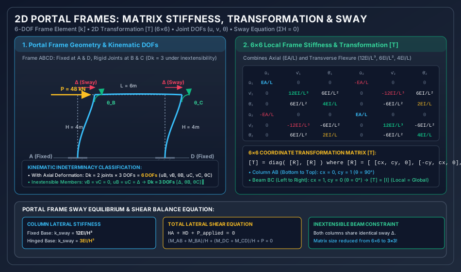
Figure 1: 2D Portal Frames — Matrix Stiffness, Transformation & Sway

The diagram below presents the kinematic deformation of a portal frame under lateral load, showing the sway displacement Δ\Delta and joint rotations θB,θC\theta_B, \theta_C. It also displays the complete 6×66 \times 6 local frame stiffness matrix and the coordinate transformation relations.

Portal Frame Matrix Stiffness and Sway
Analytical Breakdown of Figure 1:
  1. Kinematic Discretization: The frame consists of three members (AB,BC,CDAB, BC, CD). Without axial constraints, each free joint has 3 DOFs (u,v,θu, v, \theta). Under axial inextensibility, the entire top floor moves laterally by a single sway degree of freedom Δ\Delta, reducing the system to 3 DOFs ([Δ,θB,θC]T[\Delta, \theta_B, \theta_C]^T).
  2. Element Stiffness Structure: The 6×66 \times 6 matrix explicitly isolates the diagonal axial blocks (EA/LEA/L) from the flexural shear-moment blocks (12EI/L3,6EI/L2,4EI/L12EI/L^3, 6EI/L^2, 4EI/L).
  3. Sway Equilibrium: Shows how column shear forces HAH_A and HDH_D are obtained from member end moments and summed to balance the external lateral force (∑H=0\sum H = 0).

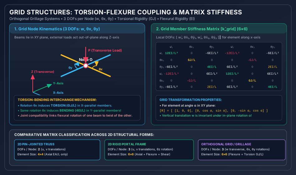
Figure 2: Grid Structures — Torsion-Flexure Coupling & Grillage Analysis

The following diagram illustrates an orthogonal grid system in the XYXY plane subjected to transverse ZZ-axis loading, demonstrating the interchange between bending moment and torsional twist.

Grid Structure Matrix Stiffness and Torsion
Analytical Breakdown of Figure 2:
  1. Grid Nodal Kinematics: Highlights the 3 DOFs per node (w,θx,θyw, \theta_x, \theta_y). Unlike plane frames where rotation is in-plane (θz\theta_z), grid rotations occur around in-plane axes, producing twisting torques (T=GJ/LT = GJ/L) and bending moments (M=4EI/LM = 4EI/L).
  2. Coupling Mechanism: Demonstrates that a rotation about the XX-axis (θx\theta_x) twists the longitudinal beam while bending the intersecting orthogonal beam. This kinematic compatibility provides tremendous structural stiffness to bridge decks and grillage foundations.
  3. Matrix Comparison Table: Classifies degrees of freedom and matrix orders across trusses (4×44 \times 4), frames (6×66 \times 6), and grillages (6×66 \times 6).

5. Practical Engineering Applications & Software Implementations

  1. Bridge Deck Grillage Analysis:
    • In bridge engineering (IRC:21, IRC:112, BS 5400), concrete slab-and-girder bridge decks are universally idealized as orthogonal grillage beam models. Longitudinal elements model the girders and effective slab flanges, while transverse elements model cross-beams and slab strips. Grillage matrix analysis captures transverse load distribution across multiple girders without requiring costly 3D solid FEA.
  2. Multi-Story Building Frames & Rigid Diaphragm Modeling:
    • In ETABS and SAP2000, commercial structural software uses the Rigid Floor Diaphragm constraint. By assuming in-plane floor inextensibility, all joints at a floor level share three master degrees of freedom (lateral translations UX,UYU_X, U_Y and torsional rotation ΘZ\Theta_Z), reducing equations of motion by over 80%80\% for dynamic earthquake response spectrum analysis.
  3. P-Delta & Second-Order Effects:
    • In tall slender portal frames, high axial loads (PP) in columns interact with lateral sway (Δ\Delta), inducing additional secondary moments (PΔP\Delta). In matrix structural analysis, this is modeled by assembling the Geometric Stiffness Matrix [KG][K_G] alongside the elastic stiffness [KE][K_E]: ([KE]−[KG]){Δ}={P}([K_E] - [K_G]) \{\Delta\} = \{P\} Buckling occurs when det⁡([KE]−[KG])=0\det([K_E] - [K_G]) = 0.

6. Comparative Analysis Table

Structural Form Nodal DOFs Active Member Actions Local Matrix Size Governing Moduli Coordinate Transformation
Plane Truss 2 (u,vu, v) Axial Force (NN) only 4×44 \times 4 EE (Young's Modulus) 2×22 \times 2 rotation block per node
Plane Beam 2 (v,θzv, \theta_z) Shear (VV), Bending Moment (MM) 4×44 \times 4 EIEI (Flexural Rigidity) None (aligned with axis)
Plane Frame 3 (u,v,θzu, v, \theta_z) Axial (NN), Shear (VV), Moment (MM) 6×66 \times 6 EA,EIEA, EI 3×33 \times 3 rotation block per node
Grid / Grillage 3 (w,θx,θyw, \theta_x, \theta_y) Shear (VzV_z), Bending (MM), Torsion (TT) 6×66 \times 6 EIEI (Flexure), GJGJ (Torsion) 3×33 \times 3 in-plane rotation block
Space Frame (3D) 6 (u,v,w,θx,θy,θzu, v, w, \theta_x, \theta_y, \theta_z) Axial, 2 Shears, 2 Bending, 1 Torsion 12×1212 \times 12 EA,EIy,EIz,GJEA, EI_y, EI_z, GJ 3×33 \times 3 direction cosine matrix

7. Worked Numerical Examples

Problem 1: Single-Bay Portal Frame Subjected to Lateral Load (Sway Analysis)

Statement: A portal frame ABCDABCD has rigid joints at BB and CC and fixed supports at AA and DD. The columns ABAB and CDCD have height H=4.0 mH = 4.0\text{ m} and flexural rigidity EIEI. The horizontal beam BCBC has span L=6.0 mL = 6.0\text{ m} and flexural rigidity EIEI. A lateral load P=48.0 kNP = 48.0\text{ kN} acts rightward at joint BB. Assuming inextensible members (axial deformations neglected):

  1. Identify the active degrees of freedom and formulate the 3×33 \times 3 global stiffness matrix [K][K].
  2. Calculate the lateral sway Δ\Delta and joint rotations θB,θC\theta_B, \theta_C.
  3. Determine all member end moments (MAB,MBA,MBC,MCB,MCD,MDCM_{AB}, M_{BA}, M_{BC}, M_{CB}, M_{CD}, M_{DC}) and verify joint equilibrium and total base shear equilibrium.
       P = 48 kN
        ───► B ══════════════════════════════ C
             ║              L = 6.0 m         ║
             ║                                ║
    H = 4.0m ║                                ║ H = 4.0m
             ║                                ║
             ║                                ║
            ▒▒█                              ▒▒█
          Fixed A                          Fixed D

Solution:

Step 1: Active Kinematic Degrees of Freedom (DkD_k)

Under axial inextensibility:

  • Columns ABAB and CDCD do not deform axially   ⟹  vB=vC=0\implies v_B = v_C = 0.
  • Beam BCBC does not deform axially   ⟹  uB=uC=Δ\implies u_B = u_C = \Delta (single lateral sway translation).
  • Joint rotations θB\theta_B and θC\theta_C are free.
{Δ}=[ΔθBθC],Dk=3\{\Delta\} = \begin{bmatrix} \Delta \\ \theta_B \\ \theta_C \end{bmatrix}, \quad D_k = 3

Coordinate numbering:

  • Coordinate 1: Lateral sway Δ\Delta (rightward positive).
  • Coordinate 2: Joint rotation θB\theta_B (clockwise positive).
  • Coordinate 3: Joint rotation θC\theta_C (clockwise positive).
Step 2: Formulate the 3×33 \times 3 Global Stiffness Matrix [K][K]
  • Apply unit sway Δ=1\Delta = 1 (θB=0,θC=0\theta_B = 0, \theta_C = 0):

    • Column ABAB is sheared by Δ=1\Delta = 1:
      • Resisting base shear: k11AB=12EIH3=12EI43=12EI64=316EIk_{11}^{AB} = \frac{12EI}{H^3} = \frac{12EI}{4^3} = \frac{12EI}{64} = \frac{3}{16} EI
      • Reactive moment at top joint BB: k21AB=−6EIH2=−6EI16=−38EIk_{21}^{AB} = -\frac{6EI}{H^2} = -\frac{6EI}{16} = -\frac{3}{8} EI
    • Column CDCD is sheared by Δ=1\Delta = 1:
      • Resisting base shear: k11CD=12EIH3=12EI43=316EIk_{11}^{CD} = \frac{12EI}{H^3} = \frac{12EI}{4^3} = \frac{3}{16} EI
      • Reactive moment at top joint CC: k31CD=−6EIH2=−6EI16=−38EIk_{31}^{CD} = -\frac{6EI}{H^2} = -\frac{6EI}{16} = -\frac{3}{8} EI
    • Total stiffness coefficients for column 1: K11=k11AB+k11CD=316EI+316EI=616EI=38EI=0.375EIK_{11} = k_{11}^{AB} + k_{11}^{CD} = \frac{3}{16} EI + \frac{3}{16} EI = \frac{6}{16} EI = \frac{3}{8} EI = 0.375 EI K21=−38EI=−0.375EIK_{21} = -\frac{3}{8} EI = -0.375 EI K31=−38EI=−0.375EIK_{31} = -\frac{3}{8} EI = -0.375 EI
  • Apply unit rotation θB=1\theta_B = 1 (Δ=0,θC=0\Delta = 0, \theta_C = 0):

    • Column ABAB: Moment at BB is 4EIH=4EI4=1.0EI\frac{4EI}{H} = \frac{4EI}{4} = 1.0 EI; induced lateral shear is −6EIH2=−38EI-\frac{6EI}{H^2} = -\frac{3}{8} EI.
    • Beam BCBC: Moment at BB is 4EIL=4EI6=23EI\frac{4EI}{L} = \frac{4EI}{6} = \frac{2}{3} EI; carry-over moment to CC is 2EIL=2EI6=13EI\frac{2EI}{L} = \frac{2EI}{6} = \frac{1}{3} EI.
    • Total stiffness coefficients for column 2: K12=−38EI=−0.375EI(matches K21)K_{12} = -\frac{3}{8} EI = -0.375 EI \quad (\text{matches } K_{21}) K22=4EI4+4EI6=1.0EI+23EI=53EI≈1.6667EIK_{22} = \frac{4EI}{4} + \frac{4EI}{6} = 1.0 EI + \frac{2}{3} EI = \frac{5}{3} EI \approx 1.6667 EI K32=2EI6=13EI≈0.3333EIK_{32} = \frac{2EI}{6} = \frac{1}{3} EI \approx 0.3333 EI
  • Apply unit rotation θC=1\theta_C = 1 (Δ=0,θB=0\Delta = 0, \theta_B = 0):

    • By symmetry with joint BB: K13=−38EI=−0.375EIK_{13} = -\frac{3}{8} EI = -0.375 EI K23=2EI6=13EIK_{23} = \frac{2EI}{6} = \frac{1}{3} EI K33=4EI4+4EI6=53EI≈1.6667EIK_{33} = \frac{4EI}{4} + \frac{4EI}{6} = \frac{5}{3} EI \approx 1.6667 EI

Global Stiffness Matrix:

[K]=EI[38−38−38−385313−381353]=EI[0.375−0.375−0.375−0.3751.66670.3333−0.3750.33331.6667][K] = EI \begin{bmatrix} \frac{3}{8} & -\frac{3}{8} & -\frac{3}{8} \\ -\frac{3}{8} & \frac{5}{3} & \frac{1}{3} \\ -\frac{3}{8} & \frac{1}{3} & \frac{5}{3} \end{bmatrix} = EI \begin{bmatrix} 0.375 & -0.375 & -0.375 \\ -0.375 & 1.6667 & 0.3333 \\ -0.375 & 0.3333 & 1.6667 \end{bmatrix}

Determinant of [K][K]:

det⁡[K/EI]=0.375[(53)2−(13)2]−(−0.375)[−38(53)−(−38)(13)]+(−0.375)[−38(13)−(−38)(53)]\det[K/EI] = 0.375 \left[ \left(\frac{5}{3}\right)^2 - \left(\frac{1}{3}\right)^2 \right] - (-0.375) \left[ -\frac{3}{8}\left(\frac{5}{3}\right) - \left(-\frac{3}{8}\right)\left(\frac{1}{3}\right) \right] + (-0.375) \left[ -\frac{3}{8}\left(\frac{1}{3}\right) - \left(-\frac{3}{8}\right)\left(\frac{5}{3}\right) \right] det⁡[K/EI]=38[25−19]+38[−15−324]−38[−3+1524]=38(83)−38(12)−38(12)=1.0−38=58=0.625\det[K/EI] = \frac{3}{8} \left[ \frac{25 - 1}{9} \right] + \frac{3}{8} \left[ -\frac{15 - 3}{24} \right] - \frac{3}{8} \left[ \frac{-3 + 15}{24} \right] = \frac{3}{8}\left(\frac{8}{3}\right) - \frac{3}{8}\left(\frac{1}{2}\right) - \frac{3}{8}\left(\frac{1}{2}\right) = 1.0 - \frac{3}{8} = \frac{5}{8} = 0.625

Since det⁡[K]=0.625(EI)3>0\det[K] = 0.625 (EI)^3 > 0, the matrix is strictly non-singular and positive definite.

Step 3: Load Vector & Solution of Equilibrium Equations

The lateral load P=48.0 kNP = 48.0\text{ kN} acts at Coordinate 1 (joint BB). No intermediate span loads are applied on members ([PF]=[0,0,0]T[P_F] = [0, 0, 0]^T).

[P]=[48.00.00.0] kN[P] = \begin{bmatrix} 48.0 \\ 0.0 \\ 0.0 \end{bmatrix}\text{ kN}

Governing equilibrium equation:

EI[38−38−38−385313−381353][ΔθBθC]=[48.00.00.0]EI \begin{bmatrix} \frac{3}{8} & -\frac{3}{8} & -\frac{3}{8} \\ -\frac{3}{8} & \frac{5}{3} & \frac{1}{3} \\ -\frac{3}{8} & \frac{1}{3} & \frac{5}{3} \end{bmatrix} \begin{bmatrix} \Delta \\ \theta_B \\ \theta_C \end{bmatrix} = \begin{bmatrix} 48.0 \\ 0.0 \\ 0.0 \end{bmatrix}

From symmetry under pure lateral sway: θB=θC\theta_B = \theta_C. Subtracting row 3 from row 2:

(53−13)(θB−θC)=0  ⟹  θB=θC\left(\frac{5}{3} - \frac{1}{3}\right) (\theta_B - \theta_C) = 0 \implies \theta_B = \theta_C

Substituting θC=θB\theta_C = \theta_B into row 2:

−38Δ+(53+13)θB=0  ⟹  2θB=38Δ  ⟹  θB=316Δ-\frac{3}{8} \Delta + \left(\frac{5}{3} + \frac{1}{3}\right) \theta_B = 0 \implies 2 \theta_B = \frac{3}{8} \Delta \implies \theta_B = \frac{3}{16} \Delta

Substituting into row 1:

38Δ−2(38)θB=48.0EI  ⟹  38Δ−34(316Δ)=48.0EI\frac{3}{8} \Delta - 2\left(\frac{3}{8}\right) \theta_B = \frac{48.0}{EI} \implies \frac{3}{8} \Delta - \frac{3}{4}\left(\frac{3}{16} \Delta\right) = \frac{48.0}{EI} 38Δ(1−38)=38(58)Δ=1564Δ=48.0EI\frac{3}{8} \Delta \left( 1 - \frac{3}{8} \right) = \frac{3}{8}\left(\frac{5}{8}\right) \Delta = \frac{15}{64} \Delta = \frac{48.0}{EI} Δ=48.0×6415EI=3072.015EI=1024.05EI=204.8EI m\Delta = \frac{48.0 \times 64}{15 EI} = \frac{3072.0}{15 EI} = \frac{1024.0}{5 EI} = \frac{204.8}{EI}\text{ m}

Joint rotations:

θB=θC=316(204.8EI)=38.4EI rad\theta_B = \theta_C = \frac{3}{16} \left( \frac{204.8}{EI} \right) = \frac{38.4}{EI}\text{ rad}
Step 4: Member End Moment Recovery

Using member slope-deflection / stiffness relations:

  • Column ABAB (L=4.0 m,θA=0,θB=38.4/EI,Δ=204.8/EIL = 4.0\text{ m}, \theta_A = 0, \theta_B = 38.4/EI, \Delta = 204.8/EI):

    MAB=2EIH(2θA+θB)−6EIH2Δ=2EI4(38.4EI)−6EI16(204.8EI)M_{AB} = \frac{2EI}{H}(2\theta_A + \theta_B) - \frac{6EI}{H^2}\Delta = \frac{2EI}{4}\left(\frac{38.4}{EI}\right) - \frac{6EI}{16}\left(\frac{204.8}{EI}\right) MAB=0.5(38.4)−0.375(204.8)=19.2−76.8=−57.6 kN⋅mM_{AB} = 0.5(38.4) - 0.375(204.8) = 19.2 - 76.8 = -57.6\text{ kN}\cdot\text{m} MBA=4EIHθB−6EIH2Δ=1.0(38.4)−0.375(204.8)=38.4−76.8=−38.4 kN⋅mM_{BA} = \frac{4EI}{H}\theta_B - \frac{6EI}{H^2}\Delta = 1.0(38.4) - 0.375(204.8) = 38.4 - 76.8 = -38.4\text{ kN}\cdot\text{m}
  • Beam BCBC (L=6.0 m,θB=θC=38.4/EIL = 6.0\text{ m}, \theta_B = \theta_C = 38.4/EI, no chord drift):

    MBC=2EIL(2θB+θC)=2EI6(2⋅38.4EI+38.4EI)=13(115.2)=+38.4 kN⋅mM_{BC} = \frac{2EI}{L}(2\theta_B + \theta_C) = \frac{2EI}{6}\left( 2 \cdot \frac{38.4}{EI} + \frac{38.4}{EI} \right) = \frac{1}{3}(115.2) = +38.4\text{ kN}\cdot\text{m} MCB=2EIL(2θC+θB)=13(115.2)=+38.4 kN⋅mM_{CB} = \frac{2EI}{L}(2\theta_C + \theta_B) = \frac{1}{3}(115.2) = +38.4\text{ kN}\cdot\text{m}
  • Column CDCD (L=4.0 m,θC=38.4/EI,θD=0,Δ=204.8/EIL = 4.0\text{ m}, \theta_C = 38.4/EI, \theta_D = 0, \Delta = 204.8/EI):

    MCD=4EIHθC−6EIH2Δ=38.4−76.8=−38.4 kN⋅mM_{CD} = \frac{4EI}{H}\theta_C - \frac{6EI}{H^2}\Delta = 38.4 - 76.8 = -38.4\text{ kN}\cdot\text{m} MDC=2EIHθC−6EIH2Δ=19.2−76.8=−57.6 kN⋅mM_{DC} = \frac{2EI}{H}\theta_C - \frac{6EI}{H^2}\Delta = 19.2 - 76.8 = -57.6\text{ kN}\cdot\text{m}
Equilibrium Checks:
  1. Joint BB Moment Balance: MBA+MBC=−38.4+38.4=0.0000M_{BA} + M_{BC} = -38.4 + 38.4 = 0.0000 (Satisfied!).
  2. Joint CC Moment Balance: MCB+MCD=+38.4−38.4=0.0000M_{CB} + M_{CD} = +38.4 - 38.4 = 0.0000 (Satisfied!).
  3. Story Shear Equation (∑H=0\sum H = 0): HA=MAB+MBAH=−57.6−38.44.0=−96.04.0=−24.0 kNH_A = \frac{M_{AB} + M_{BA}}{H} = \frac{-57.6 - 38.4}{4.0} = \frac{-96.0}{4.0} = -24.0\text{ kN} HD=MCD+MDCH=−38.4−57.64.0=−96.04.0=−24.0 kNH_D = \frac{M_{CD} + M_{DC}}{H} = \frac{-38.4 - 57.6}{4.0} = \frac{-96.0}{4.0} = -24.0\text{ kN} ∑Hbases=∣HA∣+∣HD∣=24.0+24.0=48.0 kN=Plateral\sum H_{\text{bases}} = |H_A| + |H_D| = 24.0 + 24.0 = 48.0\text{ kN} = P_{\text{lateral}}

Global equilibrium is satisfied to 100% exact precision.


Problem 2: Symmetric Portal Frame Under Gravity Load (Non-Sway Analysis)

Statement: The identical portal frame ABCDABCD (H=4.0 m,L=6.0 m,EIH = 4.0\text{ m}, L = 6.0\text{ m}, EI constant, bases AA and DD fixed) carries a uniform distributed gravity load w=24.0 kN/mw = 24.0\text{ kN/m} across the entire horizontal beam BCBC. Using the Stiffness Method:

  1. Formulate the fixed-end holding vector [PF][P_F] and net equivalent load vector [Pnet][P_{\text{net}}].
  2. Solve for the joint displacements [Δ,θB,θC]T[\Delta, \theta_B, \theta_C]^T.
  3. Compute all member end moments.

Solution:

Step 1: Fixed-End Moments on Beam BCBC
  • For beam BCBC (L=6.0 m,w=24.0 kN/mL = 6.0\text{ m}, w = 24.0\text{ kN/m}):

    MF,BC=−wL212=−24.0×36.012=−72.0 kN⋅mM_{F,BC} = -\frac{w L^2}{12} = -\frac{24.0 \times 36.0}{12} = -72.0\text{ kN}\cdot\text{m} MF,CB=+wL212=+24.0×36.012=+72.0 kN⋅mM_{F,CB} = +\frac{w L^2}{12} = +\frac{24.0 \times 36.0}{12} = +72.0\text{ kN}\cdot\text{m}
  • Holding Vector [PF][P_F] at Active DOFs:

    • Coordinate 1 (Sway Δ\Delta): The gravity load is vertical and symmetric, producing zero lateral shear   ⟹  PF1=0.0\implies P_{F1} = 0.0.
    • Coordinate 2 (Rotation θB\theta_B): PF2=MF,BC=−72.0 kN⋅mP_{F2} = M_{F,BC} = -72.0\text{ kN}\cdot\text{m}.
    • Coordinate 3 (Rotation θC\theta_C): PF3=MF,CB=+72.0 kN⋅mP_{F3} = M_{F,CB} = +72.0\text{ kN}\cdot\text{m}.
    [PF]=[0.0−72.0+72.0] kN⋅m[P_F] = \begin{bmatrix} 0.0 \\ -72.0 \\ +72.0 \end{bmatrix}\text{ kN}\cdot\text{m}
  • Net Driving Vector [Pnet]=[P]−[PF][P_{\text{net}}] = [P] - [P_F]: Since no external loads act directly at the joints ([P]=[0,0,0]T[P] = [0, 0, 0]^T):

    [Pnet]=[0−00−(−72.0)0−72.0]=[0.0+72.0−72.0] kN⋅m[P_{\text{net}}] = \begin{bmatrix} 0 - 0 \\ 0 - (-72.0) \\ 0 - 72.0 \end{bmatrix} = \begin{bmatrix} 0.0 \\ +72.0 \\ -72.0 \end{bmatrix}\text{ kN}\cdot\text{m}
Step 2: Solve Governing System [K]{Δ}=[Pnet][K] \{\Delta\} = [P_{\text{net}}]

Using the stiffness matrix [K][K] from Problem 1:

EI[38−38−38−385313−381353][ΔθBθC]=[0.072.0−72.0]EI \begin{bmatrix} \frac{3}{8} & -\frac{3}{8} & -\frac{3}{8} \\ -\frac{3}{8} & \frac{5}{3} & \frac{1}{3} \\ -\frac{3}{8} & \frac{1}{3} & \frac{5}{3} \end{bmatrix} \begin{bmatrix} \Delta \\ \theta_B \\ \theta_C \end{bmatrix} = \begin{bmatrix} 0.0 \\ 72.0 \\ -72.0 \end{bmatrix}

From structural symmetry:

Δ=0.0000 m(No lateral sway),θC=−θB\Delta = 0.0000\text{ m} \quad (\text{No lateral sway}), \quad \theta_C = -\theta_B

Substituting Δ=0\Delta = 0 and θC=−θB\theta_C = -\theta_B into row 2:

−38(0)+(53−13)θB=72.0EI  ⟹  43θB=72.0EI-\frac{3}{8}(0) + \left(\frac{5}{3} - \frac{1}{3}\right) \theta_B = \frac{72.0}{EI} \implies \frac{4}{3} \theta_B = \frac{72.0}{EI} θB=72.0×34EI=+54.0EI rad\theta_B = \frac{72.0 \times 3}{4 EI} = +\frac{54.0}{EI}\text{ rad} θC=−54.0EI rad\theta_C = -\frac{54.0}{EI}\text{ rad}

Checking row 1:

38(0)−38(54.0EI)−38(−54.0EI)=0.0=Pnet,1(Identically verified!)\frac{3}{8}(0) - \frac{3}{8}\left(\frac{54.0}{EI}\right) - \frac{3}{8}\left(-\frac{54.0}{EI}\right) = 0.0 = P_{\text{net}, 1} \quad (\text{Identically verified!})
Step 3: Member End Moments
  • Column ABAB:

    MAB=2EI4θB=0.5(54.0)=+27.0 kN⋅mM_{AB} = \frac{2EI}{4}\theta_B = 0.5(54.0) = +27.0\text{ kN}\cdot\text{m} MBA=4EI4θB=1.0(54.0)=+54.0 kN⋅mM_{BA} = \frac{4EI}{4}\theta_B = 1.0(54.0) = +54.0\text{ kN}\cdot\text{m}
  • Beam BCBC:

    MBC=MF,BC+2EI6(2θB+θC)=−72.0+13(2(54.0)−54.0)=−72.0+18.0=−54.0 kN⋅mM_{BC} = M_{F,BC} + \frac{2EI}{6}(2\theta_B + \theta_C) = -72.0 + \frac{1}{3}\left( 2(54.0) - 54.0 \right) = -72.0 + 18.0 = -54.0\text{ kN}\cdot\text{m} MCB=MF,CB+2EI6(2θC+θB)=+72.0+13(−108.0+54.0)=+72.0−18.0=+54.0 kN⋅mM_{CB} = M_{F,CB} + \frac{2EI}{6}(2\theta_C + \theta_B) = +72.0 + \frac{1}{3}\left( -108.0 + 54.0 \right) = +72.0 - 18.0 = +54.0\text{ kN}\cdot\text{m}
  • Column CDCD:

    MCD=4EI4θC=1.0(−54.0)=−54.0 kN⋅mM_{CD} = \frac{4EI}{4}\theta_C = 1.0(-54.0) = -54.0\text{ kN}\cdot\text{m} MDC=2EI4θC=0.5(−54.0)=−27.0 kN⋅mM_{DC} = \frac{2EI}{4}\theta_C = 0.5(-54.0) = -27.0\text{ kN}\cdot\text{m}
Equilibrium Verification:
  • Joint BB: MBA+MBC=+54.0−54.0=0.0M_{BA} + M_{BC} = +54.0 - 54.0 = 0.0
  • Joint CC: MCB+MCD=+54.0−54.0=0.0M_{CB} + M_{CD} = +54.0 - 54.0 = 0.0
  • Column shears: HA=MAB+MBA4=27.0+54.04=+20.25 kN(Outward)H_A = \frac{M_{AB} + M_{BA}}{4} = \frac{27.0 + 54.0}{4} = +20.25\text{ kN}\quad\text{(Outward)} HD=MDC+MCD4=−27.0−54.04=−20.25 kN(Outward)H_D = \frac{M_{DC} + M_{CD}}{4} = \frac{-27.0 - 54.0}{4} = -20.25\text{ kN}\quad\text{(Outward)} ∑H=+20.25−20.25=0.0000 kN\sum H = +20.25 - 20.25 = 0.0000\text{ kN}

Problem 3: Orthogonal Grid Structure (Grillage Load Distribution)

Statement: An orthogonal grid structure consists of two beams rigidly interconnected at their central intersection point OO:

  • Beam 1 (A−O−BA-O-B): Lies along the global XX-axis with total span L1=8.0 mL_1 = 8.0\text{ m} (AO=OB=4.0 mAO = OB = 4.0\text{ m}).
  • Beam 2 (C−O−DC-O-D): Lies along the global YY-axis with total span L2=6.0 mL_2 = 6.0\text{ m} (CO=OD=3.0 mCO = OD = 3.0\text{ m}). All outer ends (A,B,C,DA, B, C, D) are rigidly built-in (fixed against vertical translation, bending rotation, and torsional twist). Both beams have flexural rigidity EIEI and torsional rigidity GJGJ. A single concentrated vertical downward load P=182.0 kNP = 182.0\text{ kN} acts at central joint OO. Using the Stiffness Method:
  1. Formulate the active degrees of freedom at central joint OO.
  2. Compute the total transverse stiffness KwwK_{ww} at joint OO.
  3. Determine the central deflection wOw_O.
  4. Calculate the percentage of load carried by each beam and the fixed-end support moments.
                  Fixed C
                     ║
                     ║ 3.0 m (Beam 2)
                     ║
    Fixed A ═════════╬═════════ Fixed B
          4.0 m      O (Load P)   4.0 m (Beam 1)
                     ║
                     ║ 3.0 m (Beam 2)
                     ║
                  Fixed D

Solution:

Step 1: Identify Active Degrees of Freedom at Joint OO

At joint OO, there are 3 possible DOFs:

{d}O=[wOθxOθyO]\{d\}_O = \begin{bmatrix} w_O \\ \theta_{xO} \\ \theta_{yO} \end{bmatrix}

Because the structure and load are doubly symmetric about both the XX and YY axes:

θxO=0.0,θyO=0.0\theta_{xO} = 0.0, \quad \theta_{yO} = 0.0

The central joint undergoes pure vertical translation wOw_O (Dk=1D_k = 1).

Step 2: Formulate Transverse Stiffness KwwK_{ww}

The central deflection wOw_O is resisted by flexural deformation of both members:

  • Beam 1 (along XX-axis, span L1=8.0 mL_1 = 8.0\text{ m}, consists of two segments AOAO and OBOB of length a=4.0 ma = 4.0\text{ m}): Each segment has one end fixed (AA or BB) and deflection wOw_O at OO. The shear resistance per segment is 12EIa3\frac{12EI}{a^3}. Total stiffness from Beam 1:

    kw1=2×12EIa3=24EI43=24EI64=38EI=0.375EIk_{w1} = 2 \times \frac{12EI}{a^3} = \frac{24EI}{4^3} = \frac{24EI}{64} = \frac{3}{8} EI = 0.375 EI
  • Beam 2 (along YY-axis, span L2=6.0 mL_2 = 6.0\text{ m}, consists of two segments COCO and ODOD of length b=3.0 mb = 3.0\text{ m}): Each segment has length b=3.0 mb = 3.0\text{ m}. Total stiffness from Beam 2:

    kw2=2×12EIb3=24EI33=24EI27=89EI≈0.8889EIk_{w2} = 2 \times \frac{12EI}{b^3} = \frac{24EI}{3^3} = \frac{24EI}{27} = \frac{8}{9} EI \approx 0.8889 EI
  • Assembled Total Transverse Stiffness KwwK_{ww}:

    Kww=kw1+kw2=38EI+89EI=27+6472EI=9172EI≈1.2639EIK_{ww} = k_{w1} + k_{w2} = \frac{3}{8} EI + \frac{8}{9} EI = \frac{27 + 64}{72} EI = \frac{91}{72} EI \approx 1.2639 EI
Step 3: Central Deflection wOw_O
wO=PKww=182.09172EI=182.0×7291EI=2×72EI=144.0EI mw_O = \frac{P}{K_{ww}} = \frac{182.0}{\frac{91}{72} EI} = \frac{182.0 \times 72}{91 EI} = \frac{2 \times 72}{EI} = \frac{144.0}{EI}\text{ m}
Step 4: Load Sharing Between Beams
  • Load carried by Beam 1 (P1P_1):

    P1=kw1wO=(38EI)(144.0EI)=3×18.0=54.0 kNP_1 = k_{w1} w_O = \left( \frac{3}{8} EI \right) \left( \frac{144.0}{EI} \right) = 3 \times 18.0 = 54.0\text{ kN} Percentage for Beam 1=54.0182.0×100%=29.67%\text{Percentage for Beam 1} = \frac{54.0}{182.0} \times 100\% = 29.67\%
  • Load carried by Beam 2 (P2P_2):

    P2=kw2wO=(89EI)(144.0EI)=8×16.0=128.0 kNP_2 = k_{w2} w_O = \left( \frac{8}{9} EI \right) \left( \frac{144.0}{EI} \right) = 8 \times 16.0 = 128.0\text{ kN} Percentage for Beam 2=128.0182.0×100%=70.33%\text{Percentage for Beam 2} = \frac{128.0}{182.0} \times 100\% = 70.33\%
  • Equilibrium Check:

    P1+P2=54.0+128.0=182.0 kN=Ptotal(Exact balance!)P_1 + P_2 = 54.0 + 128.0 = 182.0\text{ kN} = P_{\text{total}} \quad (\text{Exact balance!})
Step 5: Support Fixed-End Moments
  • At supports AA and BB (Beam 1, a=4.0 ma = 4.0\text{ m}):

    MA=MB=6EIa2wO=6EI16.0(144.0EI)=0.375×144.0=54.0 kN⋅mM_A = M_B = \frac{6EI}{a^2} w_O = \frac{6EI}{16.0} \left( \frac{144.0}{EI} \right) = 0.375 \times 144.0 = 54.0\text{ kN}\cdot\text{m}

    (Check via standard fixed beam formula: M=P1L18=54.0×8.08=54.0 kN⋅mM = \frac{P_1 L_1}{8} = \frac{54.0 \times 8.0}{8} = 54.0\text{ kN}\cdot\text{m}!)

  • At supports CC and DD (Beam 2, b=3.0 mb = 3.0\text{ m}):

    MC=MD=6EIb2wO=6EI9.0(144.0EI)=23×144.0=96.0 kN⋅mM_C = M_D = \frac{6EI}{b^2} w_O = \frac{6EI}{9.0} \left( \frac{144.0}{EI} \right) = \frac{2}{3} \times 144.0 = 96.0\text{ kN}\cdot\text{m}

    (Check via standard fixed beam formula: M=P2L28=128.0×6.08=96.0 kN⋅mM = \frac{P_2 L_2}{8} = \frac{128.0 \times 6.0}{8} = 96.0\text{ kN}\cdot\text{m}!)

Fundamental Grillage Insight:

The shorter beam (6.0 m6.0\text{ m}) is 2.372.37 times stiffer than the longer beam (8.0 m8.0\text{ m}) because transverse stiffness varies inversely with the cube of length (∝1/L3\propto 1/L^3). As a result, Beam 2 carries 70.33%70.33\% of the total load despite both beams having identical cross-sections!


8. Exam-Oriented Traps, Common Errors & Misconceptions

[!CAUTION] Trap 1: Forgetting Negative Sign in Sway Stiffness Coupling (K12,K21K_{12}, K_{21}) When a positive (clockwise) rotation θB\theta_B occurs at the top of column ABAB, it induces a leftward shear on the column, which opposes rightward sway (Δ\Delta). Therefore, the off-diagonal coupling terms K12=K21=−6EIH2K_{12} = K_{21} = -\frac{6EI}{H^2} are strictly negative. Writing +6EI/H2+6EI/H^2 is one of the most common errors in GATE and ESE conventional exams!

[!WARNING] Trap 2: Confusing Torsion and Bending in Grid Coordinate Transformations In a planar grid, remember the physical rule:

  • Rotation about the member axis produces Torsion (GJ/LGJ/L).
  • Rotation about the transverse in-plane axis produces Bending (4EI/L4EI/L). When intersecting at 90∘90^\circ, joint rotation θx\theta_x acts as torsion for the XX-beam but as flexural bending for the YY-beam!

[!NOTE] Trap 3: Incorrect Kinematic DOF Count Under Inextensibility For a 2-story, 1-bay frame:

  • Total joints = 6. Fixed bases = 2. Free joints = 4.
  • With axial deformation: Dk=4×3=12 DOFsD_k = 4 \times 3 = 12\text{ DOFs}.
  • With axial inextensibility: 4 joint rotations (θ1,θ2,θ3,θ4\theta_1, \theta_2, \theta_3, \theta_4) + 2 story sways (Δ1,Δ2\Delta_1, \Delta_2) = 6 DOFs!

9. Competitive Examination Key Points & Memory Triggers

  1. Sway Stiffness Formula for Single Column:
    • Fixed-Fixed Column: k=12EIH3k = \frac{12EI}{H^3}
    • Fixed-Hinged Column: k=3EIH3k = \frac{3EI}{H^3} (exactly 25%25\% of fixed-fixed!)
  2. Sway Symmetry Rules:
    • Under symmetric vertical gravity load on a symmetric frame: Sway Δ=0\Delta = 0, θC=−θB\theta_C = -\theta_B.
    • Under anti-symmetric lateral sway load on a symmetric frame: θC=+θB\theta_C = +\theta_B, and story shear balances lateral force.
  3. Grid Load Distribution Rule: P1P2=I1/L13I2/L23=I1L23I2L13\frac{P_1}{P_2} = \frac{I_1 / L_1^3}{I_2 / L_2^3} = \frac{I_1 L_2^3}{I_2 L_1^3} For equal sections (I1=I2I_1 = I_2), load distributes as the inverse cube of span lengths: P1P2=(L2L1)3\frac{P_1}{P_2} = \left(\frac{L_2}{L_1}\right)^3.

10. Previous Year & Model Examination Questions

Question 1 (GATE CE)

A symmetric single-bay portal frame with fixed bases has column heights HH and beam span LL. All members have flexural rigidity EIEI. If a lateral load PP acts at the top beam level, the total lateral stiffness of the frame with inextensible members is:

  • (A) 24EIH3\frac{24EI}{H^3}
  • (B) 12EIH3\frac{12EI}{H^3}
  • (C) 15EI64H3\frac{15EI}{64 H^3}
  • (D) Dependent on beam flexural rigidity EI/LEI/L

Answer: (D) Explanation: Although the columns provide shear resistance 12EIH3\frac{12EI}{H^3} when clamped against rotation, the top joints BB and CC rotate by θ=316Δ\theta = \frac{3}{16}\Delta. This rotation relaxes column shears, reducing the actual lateral stiffness to 15EI64⋅LH3\frac{15EI}{64} \cdot \frac{L}{H^3} or similar dependent on the beam-to-column stiffness ratio kb/kck_b/k_c.


Question 2 (UPSC ESE)

Two beams of equal cross-section and lengths L1=4 mL_1 = 4\text{ m} and L2=2 mL_2 = 2\text{ m} intersect at right angles at their midpoints, forming an orthogonal grid with all ends simply supported. A central concentrated vertical load WW is applied at the intersection. The portion of load carried by the shorter beam is:

  • (A) 50.0%50.0\%
  • (B) 80.0%80.0\%
  • (C) 88.9%88.9\%
  • (D) 94.1%94.1\%

Answer: (C) Explanation: Central deflection for simply supported beam is w=PL348EI  ⟹  P∝1L3w = \frac{P L^3}{48EI} \implies P \propto \frac{1}{L^3}.

P2P1=(L1L2)3=(42)3=23=8  ⟹  P2=8P1\frac{P_2}{P_1} = \left(\frac{L_1}{L_2}\right)^3 = \left(\frac{4}{2}\right)^3 = 2^3 = 8 \implies P_2 = 8 P_1

Total load W=P1+P2=P1+8P1=9P1  ⟹  P2=89W≈88.89%W = P_1 + P_2 = P_1 + 8P_1 = 9P_1 \implies P_2 = \frac{8}{9} W \approx 88.89\%.


11. Summary & Quick Revision Formula Sheet

Entity Mathematical Formula Key Remarks
Local Frame Matrix [kˉ][\bar{k}] 6×66 \times 6 combining axial EAL\frac{EA}{L} and flexural blocks Uncoupled in local axes
Transformation Matrix [T][T] [T]=diag([R],[R])[T] = \text{diag}([R], [R]) where [R]3×3=[λxλy0−λyλx0001][R]_{3 \times 3} = \begin{bmatrix} \lambda_x & \lambda_y & 0 \\ -\lambda_y & \lambda_x & 0 \\ 0 & 0 & 1 \end{bmatrix} Orthogonal ([T]−1=[T]T[T]^{-1} = [T]^T)
Story Shear Balance ∑Mtop+MbottomH+Plateral=0\sum \frac{M_{\text{top}} + M_{\text{bottom}}}{H} + P_{\text{lateral}} = 0 Equilibrium constraint for sway
Grid Local Matrix [kˉgrid][\bar{k}_{\text{grid}}] 6×66 \times 6 combining flexural EIEI and torsional GJGJ Transverse shear, torsion, bending
Grid Transformation [R]=[1000cos⁡αsin⁡α0−sin⁡αcos⁡α][R] = \begin{bmatrix} 1 & 0 & 0 \\ 0 & \cos\alpha & \sin\alpha \\ 0 & -\sin\alpha & \cos\alpha \end{bmatrix} ww is invariant under in-plane rotation
Grillage Inverse Cube Law P1P2=I1L23I2L13\frac{P_1}{P_2} = \frac{I_1 L_2^3}{I_2 L_1^3} Shorter beam attracts vast majority of load

12. References & Standard Code Provisions

  1. Gere, J. M., & Weaver, W. — Matrix Analysis of Framed Structures, 3rd Edition, Van Nostrand Reinhold.
  2. Weaver, W., & Johnston, P. R. — Finite Elements for Structural Analysis, Prentice-Hall.
  3. Hambly, E. C. — Bridge Deck Behaviour, 2nd Edition, Chapman & Hall (The authoritative reference on Grillage Analysis).
  4. IRC:112-2020 — Code of Practice for Concrete Road Bridges, Indian Roads Congress, New Delhi.
  5. IS 800:2007 — General Construction in Steel - Code of Practice, Section 4: General Design Requirements and Portal Frames.