Flexibility Method (Force Method) and Matrix Force Transformations
In this chapter (4 topics)
On this page
- 1. Executive Summary & Foundational Concepts
- 2. Flexibility Coefficients (fij), Properties & Maxwell-Betti Reciprocity
- 2.1 Definition of Flexibility Coefficient
- 2.2 Mathematical Properties of the Flexibility Matrix [F]
- 3. Formulation of System Compatibility Equations
- 3.1 The Fundamental Compatibility Relation
- 3.2 Evaluation of Flexibility Coefficients via Virtual Work (Unit Load Method)
- 4. Member Flexibility vs. System Flexibility: Force Transformation Matrix [B]
- 4.1 Unassembled Member Flexibility Matrix [fm]
- 4.2 The Force Transformation Matrix [B]
- 4.3 The Principle of Contragredience
- 5. Vereshchagin’s Rule (Graphic Multiplication of Moment Diagrams)
- Standard Graphic Multiplication Formulas for Length L with Constant EI:
- 6. Analysis of Indeterminate Beams via Matrix Flexibility
- 6.1 Two-Span Continuous Beam with Moment Redundant (MB)
- 7. Analysis of Indeterminate Pin-Jointed Trusses
- 7.1 Inclusion of Initial Fabrication Errors and Thermal Strains
- 8. Solved Numerical Examples (Rigorous 3-Problem Set)
- Problem 1: Propped Cantilever Beam via Flexibility Matrix
- Problem 2: Two-Span Continuous Beam with Support Sinking
- Problem 3: Two-Degree Indeterminate System (Ds = 2) via Matrix Inversion
- 9. Flexibility Method vs. Stiffness Method: Comprehensive Philosophical & Practical Matrix
- 10. Common Engineering Misconceptions & Exam Pitfalls
- Misconception 1: "A flexibility coefficient fii can be zero or negative."
- Misconception 2: "Any set of Ds reaction releases produces a valid primary structure."
- Misconception 3: "The flexibility matrix is not symmetric when member cross-sections are non-prismatic."
- 11. Computational Implementation, Conditioning, and Ill-Conditioned Redundant Sets
- 11.1 Condition Number of [F]
- 11.2 Why the Stiffness Method Won the Computational Revolution
- 12. Comprehensive Summary, Master Formula Sheet & Fast-Revision Checkpoints
- Master Formula Sheet
- Fast-Revision Key Takeaways
1. Executive Summary & Foundational Concepts
In structural analysis, indeterminate systems are governed by three fundamental sets of relations: Equilibrium, Compatibility, and Constitutive (Force-Displacement) relations. Based on which set of quantities is chosen as the primary unknowns, matrix structural analysis bifurcates into two complementary dual formulations:
                               STRUCTURAL ANALYSIS MATRIX DUALITY
                                                │
                ┌───────────────────────────────┴───────────────────────────────┐
                ▼                                                               ▼
     FLEXIBILITY METHOD (FORCE METHOD)                               STIFFNESS METHOD (DISPLACEMENT METHOD)
     • Unknowns: Redundant Forces [R]                                • Unknowns: Joint Displacements [Δ]
     • Governing Size: Static Indeterminacy (Ds)                     • Governing Size: Kinematic Indeterminacy (Dk)
     • Enforces: Compatibility of Displacements                     • Enforces: Joint Equilibrium of Forces
     • Best suited when: Ds < Dk                                     • Best suited when: Dk < Ds (Modern FEA standard)
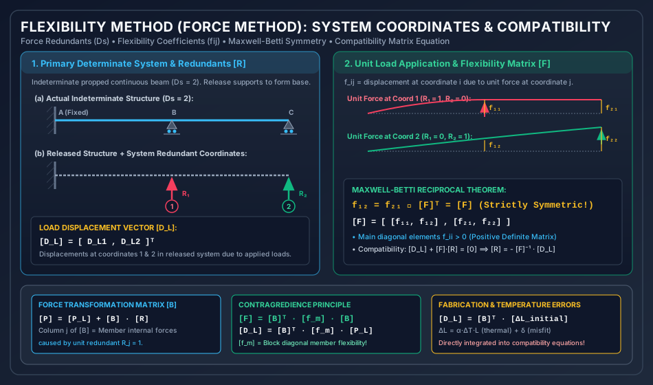
The Flexibility Method (historically termed the Method of Consistent Deformations, Force Method, or Compatibility Method) selects a set of redundant internal forces or reaction components . These redundants are released (cut or removed), transforming the original indeterminate structure into a statically determinate and stable primary structure (the released base system).
Because the release of restraints permits unphysical geometric discontinuities, the Compatibility Equations are established to ensure that the cumulative displacements at the redundant coordinates—arising from the combined effects of applied external loads, redundant forces, temperature variations, and support settlements—strictly equal the prescribed boundary conditions:
Solving this linear system yields the redundant forces , from which all remaining reactions, shear forces, and bending moments follow directly by static equilibrium.
2. Flexibility Coefficients (), Properties & Maxwell-Betti Reciprocity
2.1 Definition of Flexibility Coefficient
A flexibility coefficient is defined as:
The displacement at coordinate caused by a unit force (or unit moment) applied at coordinate , while all other coordinate forces are held at zero.
- Dimensional Units:
- Linear displacement due to unit point load: or .
- Angular rotation due to unit moment: or .
- Linear displacement due to unit moment (or rotation due to unit force): or .
2.2 Mathematical Properties of the Flexibility Matrix
- Square Matrix: If the degree of static indeterminacy is , the flexibility matrix is of order .
- Symmetry ():
According to Maxwell’s Reciprocal Deflection Theorem (and the generalized Betti’s Law), the deflection at coordinate due to a unit load at is identical to the deflection at coordinate due to a unit load at : Consequently, for a system of degree , only independent coefficients require computation. - Strictly Positive Diagonal Elements ():
A positive force applied along coordinate must produce a displacement in the same positive direction. The work done by the unit force during this displacement is: A zero or negative diagonal coefficient represents a physical instability or mechanism. - Positive Definiteness:
The total internal strain energy stored under any arbitrary redundant force vector is quadratic and strictly positive: Therefore, all eigenvalues of are real and strictly positive, and the determinant is non-zero: This guarantees that the inverse exists uniquely.
3. Formulation of System Compatibility Equations
3.1 The Fundamental Compatibility Relation
Let an indeterminate structure have static indeterminacy . Establish redundant coordinates along the lines of action of the chosen redundants .
In the released primary determinate structure:
- Let be the displacement vector at the redundant coordinates caused exclusively by external gravity/applied loads.
- Let be the flexibility matrix, where column contains the displacements produced by a unit redundant force .
- Let be the vector of prescribed support displacements (e.g., support settlement, sinkage, or rotation).
By the Principle of Superposition:
Rearranging into standard matrix form:
Premultiplying by the inverse flexibility matrix :
When supports are unyielding ():
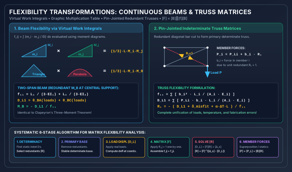
3.2 Evaluation of Flexibility Coefficients via Virtual Work (Unit Load Method)
From the Principle of Virtual Work, for any flexural structural system:
where:
- is the internal bending moment distribution in the released structure caused by a virtual unit load applied at coordinate ().
- is the internal bending moment distribution in the released structure caused by a real unit load applied at coordinate ().
Similarly, the load displacement vector evaluates as:
where is the bending moment distribution in the released structure caused by the actual external loads.
For pin-jointed trusses:
where is the axial force in member due to , and is the axial force in member due to external loads.
4. Member Flexibility vs. System Flexibility: Force Transformation Matrix
In systematic computer-oriented matrix structural analysis, flexibility analysis is decoupled into unassembled member relations and a topological connectivity transformation.
4.1 Unassembled Member Flexibility Matrix
For a discrete structure comprising elements:
- Each individual element has its own member flexibility matrix .
- For a 1D axial bar member:
- For a 2D beam element with end rotations:
- The complete unassembled member flexibility matrix is a block diagonal matrix of size :
4.2 The Force Transformation Matrix
The internal member forces () can be expressed as a linear superposition of forces caused by external loads and redundant forces:
where:
- is the vector of member internal forces in the released structure due to external loads.
- is the Force Transformation Matrix ().
- Physical Interpretation: The -th column of contains the internal forces induced across all elements when a unit redundant force is applied to the released structure.
4.3 The Principle of Contragredience
By the Principle of Virtual Work, the external work done by redundant forces equals the internal complementary work done by member forces:
Substituting :
Since this must hold for any arbitrary virtual force variation :
Now, substitute the constitutive member relation :
Comparing directly with the fundamental compatibility equation :
The Contragredience Theorem: The system flexibility matrix is generated by a congruent transformation of the unassembled member flexibility matrix using the force transformation matrix .
5. Vereshchagin’s Rule (Graphic Multiplication of Moment Diagrams)
Evaluating the integral analytically via calculus is tedious. When at least one of the two moment diagrams () is linear (which is always true for unit point loads or unit moments applied to straight elements), the integral can be solved geometrically using Vereshchagin’s Rule:
where:
- is the total area of the actual load moment diagram .
- is the ordinate of the linear diagram evaluated directly beneath the centroid of .
Standard Graphic Multiplication Formulas for Length with Constant :
| Diagram 1 () | Diagram 2 ( or ) | Value of |
|---|---|---|
| Rectangle (height ) | Rectangle (height ) | |
| Rectangle (height ) | Triangle (height ) | |
| Triangle (height ) | Triangle (height , apexes same end) | |
| Triangle (height ) | Triangle (height , apexes opposite ends) | |
| Triangle (height ) | Trapezoid (heights ) | |
| Triangle (height ) | Standard Parabola (apex midspan, height ) | |
| Trapezoid () | Trapezoid () |
6. Analysis of Indeterminate Beams via Matrix Flexibility
6.1 Two-Span Continuous Beam with Moment Redundant ()
Consider a two-span continuous beam on simple supports ( for ; for ).
- Degree of Indeterminacy: .
- Choice of Redundant: The internal bending moment at central support , .
- Released Structure: Two independent simply supported beams and .
- Coordinate 1: Relative angular rotation at support ().
Step 1: Flexibility Coefficient
Apply a unit internal hogging moment at support :
- In span , a unit moment at produces an end rotation at of .
- In span , a unit moment at produces an end rotation at of .
- Total relative rotation:
Step 2: Load Displacements
Under external loads on simply supported spans:
- Rotations at are and .
- For UDL on : .
- For concentrated load at center of : .
- Total relative rotation:
Step 3: Compatibility Equation
(Notice that clearing denominators reproduces Clapeyron’s Theorem of Three Moments exactly!)
7. Analysis of Indeterminate Pin-Jointed Trusses
For a pin-jointed truss with static indeterminacy :
- Select internal redundant bars (or redundant support reactions).
- Cut the redundant members to create the primary determinate base truss.
7.1 Inclusion of Initial Fabrication Errors and Thermal Strains
If member has:
- A fabrication error (too long by or too short by ).
- A temperature change producing free thermal strain .
The total initial non-mechanical elongation vector of the members is:
The compatibility condition becomes:
where:
Thus, the redundant forces under combined loads, temperature, and fabrication misfits are:
8. Solved Numerical Examples (Rigorous 3-Problem Set)
Problem 1: Propped Cantilever Beam via Flexibility Matrix
Statement:
A propped cantilever beam of span is rigidly fixed at and supported on a simple roller prop at . The beam carries a uniformly distributed load over its entire length. The flexural rigidity is constant throughout.
Using the Flexibility Method:
- Select the vertical prop reaction as the redundant force .
- Formulate the flexibility coefficient and load displacement .
- Solve for the prop reaction and the fixed-end moment .
Solution:
Step 1: Degree of Indeterminacy & System Coordinate
- Supports: Fixed () + Roller (). Total reactions .
- Planar equilibrium equations: .
- .
- Choose redundant: (acting vertically upward at coordinate 1).
Step 2: Released Structure & Load Displacement
The released structure is a pure cantilever beam fixed at and free at . Under UDL , the downward deflection at the free end is:
Step 3: Flexibility Coefficient
Apply a unit upward force at coordinate 1 on the released cantilever: The upward deflection at due to a unit tip point load is:
Step 4: Compatibility Equation & Solution
Assuming an unyielding prop ():
(Check standard formula: — Exact!)
Step 5: Fixed-End Bending Moment at
Taking moments about section :
(Check standard formula: — Exact!)
Problem 2: Two-Span Continuous Beam with Support Sinking
Statement:
A continuous beam has spans and with constant . Span carries a UDL , and span carries a central concentrated load .
- Choose the central support bending moment as redundant and determine .
- Compute the support reactions .
- If support sinks vertically downward by (), calculate the modified support moment .
Solution:
Step 1: Flexibility Coefficient
With redundant (unit hogging moment applied to released simply supported spans and ):
Step 2: Load Displacements in Released Spans
- Rotation at in span due to UDL :
- Rotation at in span due to point load at midspan:
- Total load displacement vector:
Step 3: Support Moment (Rigid Supports)
Step 4: Vertical Reactions
- Span :
- Span :
- Central Support Reaction:
Check equilibrium: (Verified).
Step 5: Effect of Support Sinking by
Downward settlement of central support creates chord rotations:
- In span : chord rotates clockwise by .
- In span : chord rotates counter-clockwise by .
- Relative settlement rotation:
- Modified Compatibility:
(Support sinking increased the central hogging moment from to !).
Problem 3: Two-Degree Indeterminate System () via Matrix Inversion
Statement:
A continuous beam is fixed at end , supported on a simple roller at , and supported on a simple roller at .
Span , span . .
Loads: Uniform load on span ; concentrated load at midspan of .
Using matrix flexibility with redundants (fixing moment at ) and (moment at support ):
- Assemble the flexibility matrix and load vector .
- Invert and solve for the redundant moments .
Solution:
Step 1: Flexibility Matrix Formulation
Released structure: Simply supported beam () and simply supported beam ().
- Unit redundant at coordinate 1 (End ):
- Unit redundant at coordinate 2 (Support ):
Assembled Flexibility Matrix:
Step 2: Load Displacement Vector
- In span under UDL :
- In span under point load at midspan:
- Coordinate displacements:
Step 3: Matrix Inversion & Compatibility Solution
Determinant of :
Inverse Flexibility Matrix :
Solving :
- Results:
- Fixing moment at : (sagging).
- Support moment at : (hogging).
9. Flexibility Method vs. Stiffness Method: Comprehensive Philosophical & Practical Matrix
| Characteristic / Parameter | Flexibility Method (Force Method) | Stiffness Method (Displacement Method) |
|---|---|---|
| Primary Unknowns | Forces / Redundants | Joint Displacements |
| Matrix Size | (Degree of Static Indeterminacy) | (Degree of Kinematic Indeterminacy) |
| Primary Base Structure | Determinate & stable released structure | Kinematically locked structure (all joints fixed) |
| Governing Equations | Compatibility of displacements: | Joint equilibrium of forces: |
| Matrix Properties | is symmetric, positive definite | is symmetric, positive definite, banded |
| Ease of Automation | Difficult; selection of redundants requires human judgment | Trivially automated; degrees of freedom are topological |
| Suitability for Hand Calculations | High when and is large | Tedious by hand when is large |
| Software Dominance | Obsolete in commercial FEA | Universally used in all commercial FEA software |
| Temperature & Misfits | Added directly into load displacement vector | Transformed into equivalent fixed-end force vectors |
10. Common Engineering Misconceptions & Exam Pitfalls
Misconception 1: "A flexibility coefficient can be zero or negative."
Correction: A diagonal flexibility coefficient represents the displacement along coordinate caused by a positive unit force at coordinate . Because applying a force creates positive internal strain energy (), must be strictly positive (). A non-positive value implies a kinematic mechanism or computational error.
Misconception 2: "Any set of reaction releases produces a valid primary structure."
Correction: The released structure must be both statically determinate AND geometrically stable. Releasing three parallel reactions or three concurrent reactions creates an unstable mechanism (unconstrained translation or rotation), causing to become singular ().
Misconception 3: "The flexibility matrix is not symmetric when member cross-sections are non-prismatic."
Correction: Symmetry () is an inviolable thermodynamic consequence of the Maxwell-Betti Reciprocal Theorem and the conservation of energy in linear elastic systems. It holds regardless of whether members are prismatic, tapered, curved, or composite.
11. Computational Implementation, Conditioning, and Ill-Conditioned Redundant Sets
11.1 Condition Number of
The numerical accuracy of solving depends on the condition number .
- If , the matrix is well-conditioned and stable.
- If redundant forces are chosen poorly (e.g., two redundant moments chosen at adjacent closely-spaced joints in a stiff frame), rows of become nearly linearly dependent, driving (an ill-conditioned system prone to catastrophic loss of numerical precision).
11.2 Why the Stiffness Method Won the Computational Revolution
- Algorithmic Simplicity: The stiffness method assigns degrees of freedom directly to nodes without requiring structural intuition to pick stable released bases.
- Banded Sparsity: Global stiffness matrices are narrowly banded, whereas flexibility matrices are generally dense.
12. Comprehensive Summary, Master Formula Sheet & Fast-Revision Checkpoints
Master Formula Sheet
Fast-Revision Key Takeaways
- The flexibility method treats forces as unknowns; system order equals the degree of static indeterminacy ().
- The flexibility matrix is always symmetric () and positive definite ().
- The released structure must be both determinate and stable.
- Vereshchagin’s rule allows geometric integration of moment diagrams as .
- The force transformation matrix relates member forces to redundant forces: .
- System flexibility is related to unassembled member flexibilities via .
- Initial misfits and temperature strains enter directly into the displacement compatibility vector.