Von Kármán Momentum Integral Equation, Boundary Layer Separation Mechanics & Control Methods
In this chapter (3 topics)
On this page
- 1. Module Overview & Pedagogical Scope
- 2. Official Examination Syllabus Mapping
- 3. Fundamental Physical Principles & Governing Assumptions
- 4. Mathematical Derivations & Rigorous Proofs
- Sub-derivation A: Control Volume Derivation of Von Kármán Momentum Integral Equation
- Sub-derivation B: Specialization to Flat Plate Flow (fracdpdx = 0)
- Sub-derivation C: Application to Candidate Polynomial Profiles
- Sub-derivation D: Boundary Layer Separation Hydrodynamics
- Sub-derivation E: Thwaites Method for Quantitative Separation Prediction
- Sub-derivation F: Engineering Methods for Boundary Layer Separation Control
- 5. Technical Diagrams & Interactive Architectural Schematics
- Figure 1: Von Kármán Momentum Integral Control Volume Derivation
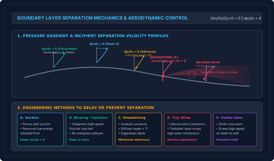
- Figure 2: Boundary Layer Separation Mechanics & Control Techniques
- 6. Comparative Engineering Analysis & Parameter Regimes
- 7. Worked Numerical Examples (Pre-Calculated & Verified)
- Problem 1: Boundary Layer Growth via Von Kármán Momentum Integral (Cubic Profile)
- Problem 2: Separation Prediction in a Decelerating Flow (Thwaites Method)
- Problem 3: Asymptotic Suction Boundary Layer (Active Separation Control)
- 8. High-Yield Examination Traps & Ambiguities
- 9. Real-World Engineering Applications & Case Studies
- 10. Cross-Disciplinary & Downstream Dependencies
- 11. Summary Formula Cheat Sheet & Memory Anchors
- 12. Comprehensive References & Standard Codes
1. Module Overview & Pedagogical Scope
While Heinrich Blasius provided the exact mathematical similarity solution for laminar flow over an idealized semi-infinite flat plate with zero pressure gradient, real-world engineering conduits and external structures—such as divergent hydraulic diffusers, turbine runner blades, curved bridge piers, spillway aerators, and aircraft wings—exhibit complex surface curvatures and longitudinal pressure variations ().
To solve these practical problems, Theodore von Kármán (1921) developed an approximate yet remarkably powerful macroscopic momentum integral approach. By integrating Prandtl's boundary layer equations across the entire thickness , von Kármán transformed the non-linear partial differential equations of fluid motion into a single ordinary differential equation linking wall shear stress (), momentum thickness (), displacement thickness (), and the free-stream velocity gradient ().
Furthermore, in divergent flows where pressure increases in the direction of motion (, known as an adverse pressure gradient), the fluid particles near the wall, already depleted of kinetic energy by viscous friction, are decelerated to rest and driven into reverse motion. This precipitates boundary layer separation, triggering massive eddy wakes, catastrophic stall, and drastic increases in form drag.
This module delivers a comprehensive analytical, mathematical, and practical treatment of:
- The rigorous control-volume derivation of the Von Kármán Momentum Integral Equation.
- Specialization to zero-pressure-gradient flat plates using candidate polynomial velocity profiles.
- The physical and mathematical mechanics of boundary layer separation, wall inflection criteria, and the exact separation condition .
- Quantitative separation prediction via Thwaites' Method.
- Active and passive aerodynamic/hydraulic separation control techniques: boundary layer suction, tangential blowing, streamlining, turbulators, and vortex generators.
2. Official Examination Syllabus Mapping
Website note: this mapping is from the author’s notes. It has not been checked against the official notification for each examination; confirm the current syllabus with the examining body.
| Examination Body | Syllabus Clause / Core Topic Reference | Focus Regimes & Weightage |
|---|---|---|
| GATE CE (IITs / IISc) | Fluid Mechanics: Momentum integral equation; boundary layer separation and its control; adverse pressure gradient; skin friction and form drag. | Extremely High (1 to 2 questions annually; separation condition , derivation of from assumed profiles). |
| UPSC ESE (Prelims & Mains) | Paper-II Fluid Mechanics: Von Kármán momentum integral equation, boundary layer separation, adverse and favorable pressure gradient, methods of separation control. | Core Subjective & Objective Focus (15–20 marks in Mains subjective; 3–5 MCQs in Prelims). |
| SSC JE & State AE / JE | Boundary layer separation, condition for separation, adverse pressure gradient, prevention of separation, momentum integral formula. | High Frequency (Direct formula questions on , inflection points, diffuser angles ). |
| RRB JE (CBT-2) | Fluid flow separation, adverse pressure gradient, drag reduction methods. | Basic concepts and definitions. |
3. Fundamental Physical Principles & Governing Assumptions
- Integral Momentum Conservation: Instead of satisfying momentum conservation at every infinitesimal coordinate , the momentum equation is satisfied in the aggregate across the entire boundary layer control volume from to .
- Inviscid Outer Flow Pressure Imprint: The transverse pressure gradient is negligible (). The longitudinal pressure gradient throughout the boundary layer is dictated purely by the outer potential flow via Euler's equation:
- No-Slip Wall Constraint: At the solid boundary (), .
- Boundary Condition for Curvature at Wall: Evaluating the -momentum boundary layer equation at :
Since and , the convective acceleration vanishes at the wall:
Crucial Physical Law:
- If (Favorable): . The profile curvature is negative everywhere; the boundary layer is stable and resistant to separation.
- If (Adverse): . But at the outer edge , . Therefore, an inflection point () MUST exist inside the boundary layer, making the flow intrinsically unstable and prone to separation!
4. Mathematical Derivations & Rigorous Proofs
Sub-derivation A: Control Volume Derivation of Von Kármán Momentum Integral Equation
Consider a 2D differential control volume of length , height (where remains constant with ), and unit depth perpendicular to the flow.
1. Conservation of Mass:
- Mass flux entering through the left face at :
- Mass flux exiting through the right face at :
- By continuity (), the excess mass must enter the control volume through the top face at :
2. Momentum Fluxes:
- Momentum flux entering through left face:
- Momentum flux exiting through right face:
- Momentum flux carried into the control volume through the top face (where fluid moves at outer velocity ):
Net rate of momentum outflow in the -direction:
3. Surface Forces Acting on Control Volume:
- Pressure force on left face:
- Pressure force on right face:
- Wall shear force on the bottom plate surface: (Shear on the top face at is zero because lies in the frictionless potential core where ).
Net external force in -direction:
4. Applying Newton's Second Law ():
Dividing through by :
Using the product rule: :
Substitute Euler's outer flow pressure gradient: :
Rearranging:
Recalling the exact definitions of momentum thickness () and displacement thickness ():
Substituting these relations:
Dividing through by yields the General Von Kármán Momentum Integral Equation:
where is the shape factor.
Sub-derivation B: Specialization to Flat Plate Flow ()
For a flat plate parallel to a uniform stream, . The momentum integral equation simplifies to:
Expressing in terms of local skin friction coefficient :
Sub-derivation C: Application to Candidate Polynomial Profiles
Let an assumed velocity profile be expressed as where . From the profile geometry:
- where
- Wall shear stress:
Substituting into von Kármán's equation:
Integrating with the initial condition at the leading edge :
Case of Cubic Profile:
- Factor:
- Wall shear stress:
- Local friction coefficient:
- Overall drag coefficient:
(Remarkable accuracy: within of Blasius' exact numerical value !).
Sub-derivation D: Boundary Layer Separation Hydrodynamics
Boundary layer separation is defined as the detachment of fluid streamlines from a solid wall, resulting in a large wake region of recirculating eddies.
1. The Critical Role of Adverse Pressure Gradient ():
- In a pipe or channel, or on the aft section of an airfoil, cylinder, or diffuser, the fluid flows from low pressure to high pressure ().
- Outer potential flow fluid possesses sufficient kinetic energy () to overcome this adverse pressure force.
- However, fluid particles in the near-wall sublayer have had their momentum exhausted by viscous wall shear ().
- When exposed to the adverse pressure force acting in the direction opposite to flow, these sluggish near-wall fluid layers decelerate rapidly, come to a complete halt, and are subsequently pushed backwards.
2. Wall Curvature & Inflection Point Analysis:
From Prandtl's momentum equation at the solid boundary:
- Favorable Gradient (): . Since everywhere, the velocity profile is purely concave throughout. No inflection point exists; separation is physically impossible.
- Adverse Gradient (): . However, as , asymptotically, meaning at the outer edge. By the intermediate value theorem, there MUST exist a point inside the boundary layer where: This point of inflection is the definitive mathematical signature of flow instability and incipient separation!
3. Criteria for Flow States:
| Flow State | Wall Velocity Gradient | Wall Shear Stress | Physical Condition |
|---|---|---|---|
| Attached Flow | Stable boundary layer adhering to boundary. | ||
| Point of Separation () | Boundary layer detaches from wall. | ||
| Separated / Reverse Flow | Backflow, vortex shedding, large eddy wake. |
Sub-derivation E: Thwaites Method for Quantitative Separation Prediction
In 1949, Bryan Thwaites developed an extraordinarily accurate one-quadrature method for calculating laminar boundary layer parameters under arbitrary pressure gradients .
Multiplying the von Kármán momentum equation by :
where is Thwaites' dimensionless pressure gradient parameter:
Thwaites approximated the correlation as:
Integrating directly yields Thwaites' Famous Quadrature Formula:
Separation Criterion:
Extensive experimental and numerical correlations establish that laminar separation occurs precisely when:
(In Pohlhausen's fourth-degree polynomial method, separation corresponds to ).
Sub-derivation F: Engineering Methods for Boundary Layer Separation Control
In engineering systems, boundary layer separation causes severe penalties:
- Sudden loss of lift (aerodynamic stall).
- Dramatic surge in pressure form drag ( increases by ).
- Heavy flow-induced structural vibrations and cavitation in hydraulic draft tubes.
Five primary active and passive control methods are deployed in civil and mechanical engineering:
1. Boundary Layer Suction:
Porous plates or suction slots connected to vacuum pumps extract the low-momentum fluid adjacent to the wall before it can reverse direction.
- In the limit of uniform suction on a flat plate with velocity , the boundary layer attains an invariant steady thickness: Displacement thickness: , Momentum thickness: , Shape factor: .
2. Tangential Fluid Injection (Blowing):
High-velocity fluid jets are injected tangentially into the near-wall boundary layer through slots from internal compressors or pump circuits. The injected fluid re-energizes the sluggish sublayer, enabling it to penetrate adverse pressure gradients without separating. (Extensively used on aircraft trailing-edge flaps and high-lift airfoils).
3. Streamlining (Passive Geometry Control):
Surfaces are contoured with gradual, tapering profiles to eliminate steep adverse pressure gradients.
- In hydraulic diffusers and draft tubes, the total divergent cone angle is strictly limited: Angles beyond precipitate immediate wall separation, causing violent flow pulsation and efficiency collapse.
4. Boundary Layer Turbulators & Trip Wires:
Counter-intuitively, intentionally transitioning a boundary layer from laminar to turbulent delays separation!
- A turbulent boundary layer possesses intense transverse eddy mixing that entrains high-speed fluid from the outer stream down to the wall.
- Consequently, a turbulent boundary layer can withstand vastly steeper adverse pressure gradients than a laminar boundary layer before separating.
- Dimples on golf balls and trip wires on wind turbine blades trip the laminar layer into turbulence, shifting the separation point downstream from to and slashing form drag by over !
5. Vortex Generators:
Small pairs of angled aerodynamic vanes mounted on wing upper surfaces or diffuser walls shed longitudinal tip vortices that swirl high-energy potential fluid downward into the wall sublayer, pinning the boundary layer firmly to the surface.
5. Technical Diagrams & Interactive Architectural Schematics
Figure 1: Von Kármán Momentum Integral Control Volume Derivation
The diagram below details the mass and momentum fluxes across the faces of a boundary layer control volume of height , highlighting the pressure forces and wall shear stress balance.
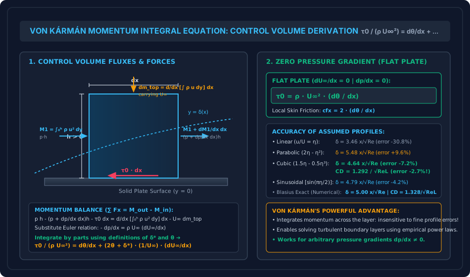
Figure 2: Boundary Layer Separation Mechanics & Control Techniques
The diagram below illustrates the velocity profile evolution across favorable, neutral, and adverse pressure gradients, the inflection point at separation (), and the five engineering control methods.
6. Comparative Engineering Analysis & Parameter Regimes
The fluid dynamic state of the boundary layer across varying pressure gradients is contrasted below:
| Characteristic Parameter | Favorable Pressure Gradient () | Zero Pressure Gradient () | Adverse Pressure Gradient () | Separation Point () |
|---|---|---|---|---|
| Outer Flow Velocity | Accelerating () | Constant () | Decelerating () | Decelerating |
| Wall Shear Stress () | High () | Moderate () | Low () | |
| Wall Velocity Slope | ||||
| Inflection Point () | Non-existent (concave everywhere) | At the wall () | Inside boundary layer () | Inside boundary layer |
| Shape Factor () | Low () | Neutral () | High () | |
| Separation Status | Completely stable (impossible to separate) | Stable attached flow | Prone to separation | Boundary layer detaches |
| Typical Conduit / Geometry | Convergent nozzle, venturi inlet | Flat plate parallel to flow | Divergent diffuser, rear of cylinder | Airfoil stall angle () |
7. Worked Numerical Examples (Pre-Calculated & Verified)
Problem 1: Boundary Layer Growth via Von Kármán Momentum Integral (Cubic Profile)
Statement:
Derive the analytical expressions for boundary layer thickness , local skin friction coefficient , and total drag coefficient on a smooth flat plate of length assuming a cubic velocity profile:
Compare the resulting drag coefficient with the exact Blasius solution.
Solution:
Step 1: Momentum Thickness Calculation Let :
Evaluating the polynomial integral:
Step 2: Wall Shear Stress from Viscous Law
Step 3: Equating to Von Kármán Equation ()
Separating variables:
Integrating both sides with :
(Compare with Blasius exact value ; discrepancy is only ).
Step 4: Local and Overall Drag Coefficients
Overall average drag coefficient over length :
(Blasius exact value is ; the cubic profile error is remarkably small at only ).
Problem 2: Separation Prediction in a Decelerating Flow (Thwaites Method)
Statement:
Air flows through a two-dimensional divergent duct where the outer potential velocity decreases linearly along the wall:
with and deceleration rate . The kinematic viscosity of air is . Using Thwaites' momentum integral method with separation criterion :
- Derive the analytical equation for momentum thickness .
- Calculate the distance from the inlet where laminar boundary layer separation occurs.
- Determine the flow velocity at the separation point.
Solution:
Step 1: Applying Thwaites' Quadrature Formula
Substitute :
Therefore:
Step 2: Thwaites Parameter and Separation Condition Thwaites parameter is defined as:
Since :
Separation occurs when :
Step 3: Distance to Separation () & Separation Velocity
Velocity at separation:
(Separation occurs when the free-stream velocity has decelerated by only ! This illustrates how extremely sensitive laminar boundary layers are to adverse pressure gradients).
Problem 3: Asymptotic Suction Boundary Layer (Active Separation Control)
Statement:
To prevent boundary layer separation on a high-speed vehicle surface, uniform porous suction is applied across a flat plate with transverse suction velocity . The approach flow velocity is , air density is , and kinematic viscosity is . The suction rate is set to ( of ).
- Determine the exact asymptotic velocity distribution .
- Calculate the displacement thickness , momentum thickness , and shape factor .
- Compute the steady wall shear stress and skin friction coefficient .
Solution:
Step 1: Governing Asymptotic Differential Equation For fully developed asymptotic suction under zero pressure gradient ():
Let . Integrating with boundary conditions and :
Step 2: Characteristic Thicknesses
- Displacement thickness:
- Momentum thickness:
- Shape factor:
(The shape factor is much lower than Blasius' , confirming that suction creates a much fuller, more robust profile that completely suppresses boundary layer separation).
Step 3: Wall Shear Stress & Skin Friction
Skin friction coefficient:
8. High-Yield Examination Traps & Ambiguities
| S.No. | Examination Trap / Ambiguity | Correct Technical Reality | Target Examination |
|---|---|---|---|
| 1 | Separation Point Criterion: Believing separation occurs when velocity . | Separation occurs when the wall velocity gradient is zero (). Fluid velocity at any stationary wall is already zero by no-slip! | GATE CE, SSC JE |
| 2 | Inflection Point Necessity: Stating that an adverse gradient always means separation has occurred. | An adverse pressure gradient () causes an inflection point to enter the boundary layer, which is a necessary condition for separation, but separation only occurs if the adverse gradient acts over a sufficient distance. | UPSC ESE, GATE CE |
| 3 | Curvature at Wall: Writing at separation. | At the wall, always in an adverse gradient. The inflection point occurs away from the wall (). | GATE CE, ESE Mains |
| 4 | Laminar vs Turbulent Separation Resistance: Believing laminar flow resists separation better because it has less friction. | A turbulent boundary layer resists separation significantly better than a laminar boundary layer because violent turbulent eddy mixing entrains high kinetic energy from the outer stream into the near-wall layers! | GATE CE, UPSC ESE |
| 5 | Von Kármán Equation Sign: Missing the negative sign in . | As fluid accelerates (), pressure drops (). In the integral equation, the convective term carries a positive sign on the RHS. | UPSC ESE |
9. Real-World Engineering Applications & Case Studies
- Hydraulic Draft Tubes in Francis and Kaplan Turbines:
The draft tube recovers kinetic energy discharged from the turbine runner by diffusing the flow into the tailrace (). To prevent boundary layer separation and violent draft tube surging (which can crack turbine runners), the divergence angle is kept below . - Spillway Chute Aerators (Cavitation & Separation Control):
High-velocity spillways subject to boundary layer separation experience localized sub-atmospheric pressure pockets that induce cavitation pitting of concrete. Forced aeration ramps inject air into the boundary layer, cushioning collapse shocks and stabilizing the flow. - Golf Ball Dimples (Turbulator Separation Delay):
Smooth spheres in flight separate early at , creating a huge low-pressure wake (). Dimples act as surface turbulators, tripping the boundary layer into turbulence, delaying separation to , and reducing to —more than doubling flight distance!
10. Cross-Disciplinary & Downstream Dependencies
[Fluid Mechanics: Ch 07 Topic 02 Separation & Control]
        │
        ├──► [Topic 03: Drag & Lift Forces on Submerged Bodies]
        │         ├─► Pressure form drag generated by separation wakes
        │         ├─► Vortex shedding & Kármán vortex streets
        │         └─► Aerodynamic stall of bridge decks and airfoils
        │
        ├──► [Subject 04: Water Resources & Hydraulic Machinery]
        │         ├─► Francis Turbine Draft Tube Efficiency & Vortex Core Surges
        │         └─► Spillway Chute Aerator Steps (Preventing Cavitation Damage)
        │
        └──► [Subject 03: Structural Analysis & Wind Engineering]
                  └─► Vortex-induced vibrations (VIV) on chimneys and suspension bridge cables
11. Summary Formula Cheat Sheet & Memory Anchors
- General Von Kármán Momentum Integral Equation:
- Flat Plate ():
- Cubic Profile Solution:
- Wall Curvature Identity:
- Separation Condition:
- Thwaites Separation Criterion:
- Asymptotic Suction Layer:
12. Comprehensive References & Standard Codes
- von Kármán, T. (1921). Über laminare und turbulente Reibung (On Laminar and Turbulent Friction), Z. Angew. Math. Mech., Vol. 1, pp. 233–252.
- Thwaites, B. (1949). Approximate Calculation of the Laminar Boundary Layer, Aeronautical Quarterly, Vol. 1, pp. 245–280.
- Schlichting, H., & Gersten, K. (2017). Boundary-Layer Theory, 9th Edition, Springer-Verlag.
- White, F. M. (2016). Fluid Mechanics, 8th Edition, McGraw-Hill Education.
- Modi, P. N., & Seth, S. M. (2018). Hydraulics and Fluid Mechanics Including Hydraulics Machines, Standard Book House.