Conservation of Mass & 3D Continuity Equation in Cartesian and Cylindrical Coordinates
In this chapter (5 topics)
On this page
- 1. Topic Metadata Table
- 2. Executive Summary
- 3. Reynolds Transport Theorem (RTT) & Physical Law of Conservation of Mass
- 3.1 Reynolds Transport Theorem Statement
- 3.2 Conservation of Mass Formulation
- 4. Derivation of 3D Continuity Equation in Cartesian Coordinates
- 4.1 Mass Inflow and Outflow Rates in the x-Direction
- 4.2 Mass Inflow and Outflow Rates in y and z Directions
- 4.3 Rate of Mass Accumulation Inside the Element
- 4.4 Global Balance & Differential Equation
- 4.5 Substantial Derivative (Lagrangian Tracking) Form
- 5. Derivation & Formulation in Cylindrical Coordinates
- 5.1 Coordinate Definition & Differential Volume
- 5.2 Radial Mass Flux Derivation
- 5.3 Azimuthal and Axial Mass Fluxes
- 5.4 Complete Cylindrical Continuity Equation
- 5.5 Important Special Cases in Cylindrical Coordinates
- 6. Incompressible Flow Condition & Solenoidal Velocity Fields
- 6.1 Strict Definition of Incompressibility
- 6.2 Physical Meaning of Solenoidal Fields
- 6.3 Incompressibility vs. Stealiness Matrix
- 7. One-Dimensional Pipe Flow & Branching Networks
- 7.1 Mass and Volumetric Discharge
- 7.2 Pipe Junctions & Bifurcation Networks
- 8. Visual Diagrams & Architectural Schematics
- 8.1 3D Differential Control Volume & Cartesian Flux Balance
- 8.2 Cylindrical Coordinate Element & Branching Pipe Network
- 9. Step-by-Step Numerical Problems with Complete Calculations
- Problem 1: Examination of a 3D Incompressible Velocity Field & Missing Component Determination
- Problem 2: Axisymmetric Seepage Flow in Cylindrical Coordinates
- Problem 3: Pipe Bifurcation Network & Conical Diffuser Sizing
- 10. High-Yield Exam Pitfalls, Traps & Shortcuts
- 11. Multi-Exam Question Bank (GATE, ESE, SSC JE, State AE, RRB JE)
- Question 1 (GATE CE — Analytical)
- Question 2 (UPSC ESE Paper-II — Descriptive / Analytical)
- Question 3 (SSC JE — Conceptual)
- Question 4 (State PSC AE — Numerical)
- Question 5 (RRB JE — Direct Formula)
- 12. Comprehensive Summary, Formula Cheatsheet & Academic References
- 12.1 Formula Cheatsheet
- 12.2 Academic & Standard References
1. Topic Metadata Table
| Field | Detail |
|---|---|
| Subject | Fluid Mechanics & Hydraulic Machinery (Subject 07) |
| Chapter | Chapter 03: Fluid Kinematics |
| Topic Code | FM-03-02 |
| Topic Title | Conservation of Mass & 3D Continuity Equation in Cartesian and Cylindrical Coordinates |
| Prerequisites | FM-03-01 (Lagrangian & Eulerian Descriptions, Flow Classification, Streamlines & Pathlines), Vector Calculus (Divergence Operator, Gauss Divergence Theorem) |
| Target Examinations | GATE CE, UPSC ESE (Paper-II), SSC JE, State PSC AE/JE, RRB JE |
| Knowledge Level | Fundamental Derivation to Advanced Analytical & Numerical Design |
| IS / IRC / Standard Codes | IS 4880 (Code of practice for design of tunnels, hydraulic aspects), IS 2951 (Methods for measurement of fluid flow) |
| Key Formulae | , , , |
2. Executive Summary
The Continuity Equation is the exact mathematical statement of the fundamental physical law of Conservation of Mass applied to a fluid flow field. Matter can neither be created nor destroyed in a non-relativistic continuum; consequently, the net rate at which mass enters any arbitrary control volume must precisely balance the net rate of mass outflow plus the instantaneous rate of mass accumulation within that volume.
In fluid mechanics, this conservation principle can be formulated either globally (integral form via the Reynolds Transport Theorem) or locally at every infinitesimal continuum point (differential form). In Cartesian coordinates , the general unsteady compressible continuity equation is:
Using the material (substantial) derivative , this transforms compactly into:
For an incompressible fluid (where fluid parcel density remains invariant along its motion, , universally applicable to water in civil engineering hydraulics), the continuity equation simplifies strictly to the solenoidal condition:
Crucially, incompressible flow does not require steady flow. Even in highly unsteady flow regimes (such as water hammer precursors or tidal surges), if the fluid density is constant, holds at every spatial coordinate at every instant of time. For axisymmetric systems—such as round pipes, wellbore radial seepage, vortices, and centrifugal pumps—the continuity equation is transformed into cylindrical coordinates , where the radial velocity term acquires a geometric curvature metric . In one-dimensional pipe hydraulics, integrating across cross-sectional streamlines yields the familiar volumetric discharge conservation , governing conduit bifurcations, diffusers, and pipe distribution networks.
3. Reynolds Transport Theorem (RTT) & Physical Law of Conservation of Mass
To establish continuity rigorously, we bridge the Lagrangian system (a fixed collection of fluid matter of constant mass ) and the Eulerian control volume (a fixed spatial region bounded by a control surface ).
3.1 Reynolds Transport Theorem Statement
Let be any extensive fluid property, and let be the corresponding intensive property (property per unit mass). The Reynolds Transport Theorem states:
where:
- is the outward-pointing unit normal vector to the control surface ,
- is the normal velocity component across (positive for efflux, negative for influx).
3.2 Conservation of Mass Formulation
For mass conservation, the extensive property is total mass, , so . By Newton's continuum postulate, the mass of a closed system is strictly invariant in time:
Substituting into the Reynolds Transport Theorem gives the Integral Form of Continuity:
Physical Interpretation:
- : Time rate of mass accumulation inside the control volume.
- : Net mass efflux rate (outflow rate minus inflow rate) through the boundary control surface.
By applying the Gauss Divergence Theorem to the surface integral, converting the surface flux into a volume integral of divergence:
Assuming the control volume is fixed in space, the time derivative enters the integral as a partial derivative:
Because this equality must hold for any arbitrary, infinitesimally small control volume , the integrand must vanish identically everywhere:
4. Derivation of 3D Continuity Equation in Cartesian Coordinates
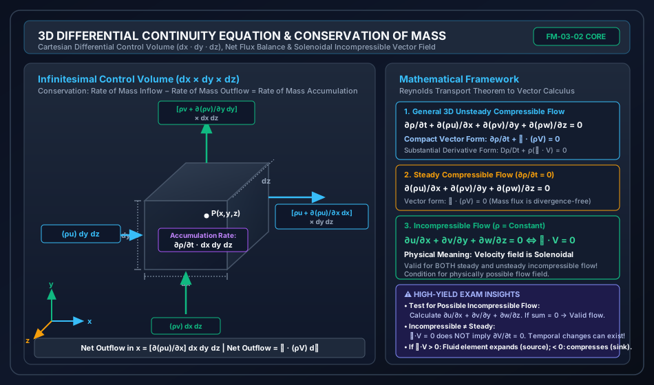
Consider an infinitesimal rectangular control volume of differential dimensions , , and centered at spatial coordinates . The total volume of this differential element is .
                    ┌───────────────────────────┐
                   /                           /│
                  /                           / │
                 ┌───────────────────────────┐  │
                 │                           │  │ dy
   流入 (Inflow) │          P(x,y,z)         │  │
   ───(ρu)dy dz──>                           │  ├───────> [ρu + ∂(ρu)/∂x dx] dy dz
                 │                           │ /  Efflux (Outflow)
                 │                           │/ dz
                 └───────────────────────────┘
                              dx
4.1 Mass Inflow and Outflow Rates in the -Direction
At the left face perpendicular to the -axis, situated at :
At the right face situated at :
The net mass outflow rate across the -faces is:
4.2 Mass Inflow and Outflow Rates in and Directions
Similarly, across the bottom and top faces perpendicular to the -axis:
Across the back and front faces perpendicular to the -axis:
Summing all three spatial dimensions gives the total net rate of mass outflow:
4.3 Rate of Mass Accumulation Inside the Element
The mass contained within the differential element at time is:
The instantaneous rate of mass increase (accumulation) inside the fixed element is:
4.4 Global Balance & Differential Equation
By conservation of mass:
Dividing throughout by the differential volume :
4.5 Substantial Derivative (Lagrangian Tracking) Form
Expanding the spatial divergence terms by product rule:
Substituting this into the continuity equation:
Recognizing that the local plus convective derivative of density is the material derivative :
This form reveals that the divergence of velocity is directly proportional to the relative rate of volumetric expansion (dilatation rate) of a fluid parcel:
5. Derivation & Formulation in Cylindrical Coordinates
For axisymmetric or rotating geometries—including well hydraulics, groundwater radial drawdown, circular tunnels, conduits, pipe flow, and turbomachinery—Cartesian coordinates become algebraically cumbersome. We employ cylindrical coordinates .
5.1 Coordinate Definition & Differential Volume
- : Radial distance from the -axis ().
- : Azimuthal (polar) angle in the - plane ().
- : Axial distance along the cylinder axis ().
- Velocity vector: .
The differential element is bounded by faces at and , and , and and .
- Face area normal to : .
- Face area normal to : .
- Face area normal to : .
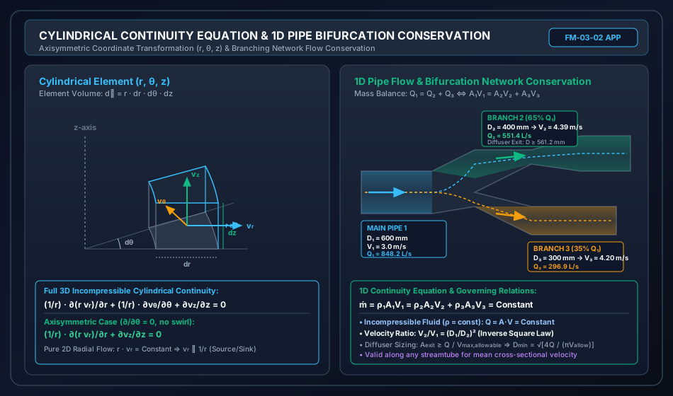
- Differential element volume:
5.2 Radial Mass Flux Derivation
Mass entering across the inner cylindrical face at radius :
Mass leaving across the outer cylindrical face at radius :
The net outflow rate in the radial direction is:
5.3 Azimuthal and Axial Mass Fluxes
Across the azimuthal faces and :
Across the axial faces and :
5.4 Complete Cylindrical Continuity Equation
Equating the net outflow to the negative rate of mass accumulation :
For incompressible flow ():
Expanding the first term:
Thus, an equivalent form is:
5.5 Important Special Cases in Cylindrical Coordinates
-
Axisymmetric Flow (): When flow is completely independent of the circumferential angle (e.g., flow in straight circular pipes, axial jets, radial well extraction):
-
Pure 2D Planar Radial Flow ():
- : Radial Source (fluid originating at axis ).
- : Radial Sink (well pumping / groundwater extraction).
- Exam Hallmark: Unlike Cartesian 1D flow where velocity must be constant (), in 2D radial cylindrical flow, continuity requires velocity to vary inversely with radial distance ().
6. Incompressible Flow Condition & Solenoidal Velocity Fields
6.1 Strict Definition of Incompressibility
Incompressibility does not simply mean that the density field is uniform everywhere. It means that the density of any specific fluid particle does not change as it traverses the flow field:
From , if and , it follows immediately that:
A vector field whose divergence is zero everywhere is known mathematically as a Solenoidal Vector Field.
6.2 Physical Meaning of Solenoidal Fields
- No Volumetric Dilatation: The volumetric strain rate (rate of change of volume per unit volume) of an infinitesimal fluid element is identically zero: A fluid parcel can deform, shear, elongate, rotate, and flatten, but its volume remains rigorously invariant.
- Absence of Interior Monopoles: There are no internal fluid creation points (sources, ) or annihilation points (sinks, ).
- Streamtube Flux Conservation: Streamlines cannot terminate in the interior of the flow field. They either form closed loops, extend to boundaries, or run to infinity. The volumetric flow rate passing through any cross-section of a streamtube is strictly constant.
6.3 Incompressibility vs. Stealiness Matrix
| Flow Condition | Compressibility () | Mathematical Expression | Example in Civil Engineering |
|---|---|---|---|
| Steady Incompressible | , | , | Steady pipe discharge, open-channel uniform flow in aqueducts |
| Unsteady Incompressible | , | , | Surge tank oscillations, valve closure transient prior to elastic wave reflection, tidal sluice operation |
| Steady Compressible | , | , | Gas transmission pipelines, high-velocity ventilation ducts in long railway tunnels |
| Unsteady Compressible | Water hammer acoustic pressure waves (where bulk modulus and pipe elasticity govern), blast waves |
7. One-Dimensional Pipe Flow & Branching Networks
When fluid flows through rigid pipes, conduits, or closed canals, cross-sectional gradients can be integrated out, leaving a one-dimensional formulation in terms of the bulk average velocity :
7.1 Mass and Volumetric Discharge
- Mass Flow Rate:
- Volumetric Flow Rate (Discharge):
For steady flow through a single conduit of variable cross-section:
For an incompressible liquid ():
For circular conduits of internal diameters and :
Velocity scales inversely with the square of the diameter. Halving the pipe diameter quadruples the mean flow velocity ().
7.2 Pipe Junctions & Bifurcation Networks
At any pipe junction (nodal manifold), conservation of mass requires the algebraic sum of mass flow rates to vanish:
For incompressible water flow:
For a bifurcating main pipe (1) dividing into two parallel delivery branches (2 and 3):
8. Visual Diagrams & Architectural Schematics
8.1 3D Differential Control Volume & Cartesian Flux Balance
The following technical schematic illustrates an infinitesimal fluid element at point , showing mass inflow and outflow rates across orthogonal faces, net flux balance, and formulation into the divergence-free solenoidal condition.
8.2 Cylindrical Coordinate Element & Branching Pipe Network
The schematic below presents the cylindrical coordinate differential element with radial curvature considerations, alongside a 1D pipe bifurcation network demonstrating volumetric flow conservation across branches and diffuser transitions.
9. Step-by-Step Numerical Problems with Complete Calculations
Problem 1: Examination of a 3D Incompressible Velocity Field & Missing Component Determination
Problem Statement: A steady incompressible flow field has velocity components given by:
- Determine whether a two-dimensional flow field is possible with these two components alone.
- Using the 3D continuity equation, determine the most general form of the third velocity component such that the flow field is physically possible.
- If on the plane , evaluate the velocity vector and its absolute magnitude at the point .
Step 1: Check 2D Incompressible Continuity
For an incompressible flow in the - plane, continuity requires:
Differentiating the given velocity components:
Summing the derivatives:
Conclusion: The sum is identically zero everywhere in the field. Therefore, a 2D flow field is theoretically possible if .
Step 2: Formulate General 3D Component
In 3D Cartesian coordinates, continuity requires:
Substituting the partial derivatives:
Integrating with respect to :
where is any arbitrary differentiable function of and , completely independent of .
Step 3: Evaluate Specific Boundary Condition and Point Values
Given the boundary condition:
Since , does not vary with . Therefore:
Now, evaluate the velocity components of the stated flow field (, , ) at the point :
- Velocity Vector at :
- Resultant Velocity Magnitude:
Problem 2: Axisymmetric Seepage Flow in Cylindrical Coordinates
Problem Statement: In a radial collector well system installed in an unconfined sand aquifer, the seepage flow is axisymmetric ().
- Prove that any purely radial 2D flow field of the form (where is a well discharge constant) identically satisfies the incompressible continuity equation.
- In a vertical recharge well, a simultaneous downward axial velocity is measured as , where is a vertical drainage rate constant. Assuming no swirl (), derive the governing expression for the radial velocity component if at the centerline .
- Compute the radial velocity at a distance from the well centerline.
Step 1: Verification of Pure Radial Incompressible Flow
In cylindrical coordinates with and , the continuity equation reduces to:
Substitute :
Differentiating with respect to :
Thus:
The continuity equation is identically satisfied for all . Q.E.D.
Step 2: Derivation with Combined Axial Velocity
The axisymmetric continuity equation is:
Given , compute the axial gradient:
Substitute into the continuity equation:
Multiply by :
Integrate both sides with respect to :
Divide by :
Apply the boundary condition at the centerline: at , must remain finite and physically bounded (no infinite singularity at the axis). Therefore, the integration constant must vanish:
Hence, the radial velocity profile is:
Step 3: Numerical Computation at
With :
At :
Physical Interpretation: Fluid is drawn radially inward toward the drainage column at an acceleration proportional to radius, balancing the downward vertical drainage flux.
Problem 3: Pipe Bifurcation Network & Conical Diffuser Sizing
Problem Statement: A main feeder water supply pipeline of diameter conveys water at a bulk velocity of . At a distribution junction, the pipeline bifurcates into two branches, Pipe 2 and Pipe 3:
- Branch Pipe 2 has a diameter of and carries of the total incoming discharge.
- Branch Pipe 3 has a diameter of and carries the remaining of the incoming discharge.
- At the termination of Branch Pipe 2, water enters a treatment sedimentation basin through a conical diffuser. To prevent scouring and flocs breakup, the discharge velocity exiting the diffuser must not exceed .
Calculate:
- The total volumetric discharge in the main pipe (in and ).
- The discharge () and mean velocities () in each branch pipe.
- The minimum required exit diameter of the conical diffuser.
Step 1: Main Pipeline Volumetric Discharge
Cross-sectional area of Main Pipe 1:
Total discharge:
Step 2: Branch Discharges and Flow Velocities
For Branch 2 ( of ):
Cross-sectional area of Branch 2:
Mean velocity in Branch 2:
For Branch 3 ( of ):
Cross-sectional area of Branch 3:
Mean velocity in Branch 3:
Verification of mass conservation:
Step 3: Conical Diffuser Sizing
At the diffuser exit, continuity requires:
To satisfy :
Relating area to diameter:
(Note: If calculated for at , ). For Branch 2 entering the basin:
10. High-Yield Exam Pitfalls, Traps & Shortcuts
- Trap: Confusing Incompressible with Steady Flow:
- Trap: Students often assume that implies the flow is steady ().
- Correction: is solely the condition of incompressibility (). An unsteady flow of water (e.g., accelerating flow in a pipe during valve opening) satisfies perfectly, while .
- Trap: Cartesian vs. Cylindrical 1D Radial Flow Velocity Decay:
- Cartesian 1D: . Velocity cannot change along the flow path without cross-flow.
- Cylindrical 2D Radial: . Velocity naturally decays inversely with radius () due to the spreading geometric perimeter ().
- Trap: Forgetting the Density Derivative in Compressible Continuity:
- In compressible flow questions (e.g., high-speed air tunnel or gas pipeline), is invalid. One must use .
- Shortcut: Quick Divergence Test for Possible Flow Field:
- To check if a velocity field is physically possible for an incompressible fluid:
- If : Valid, physically possible incompressible flow field.
- If : Invalid for incompressible flow (represents an unphysical mass leak or requires density variation).
- To check if a velocity field is physically possible for an incompressible fluid:
- Trap: Sign Convention of Divergence:
- : Net mass outflow exceeds inflow; the fluid parcel is expanding in volume (source behaviour).
- : Net mass inflow exceeds outflow; fluid parcel is contracting/compressing (sink behaviour).
11. Multi-Exam Question Bank (GATE, ESE, SSC JE, State AE, RRB JE)
Question 1 (GATE CE — Analytical)
The velocity vector for a 2D incompressible fluid flow is given by:
where are non-zero constants. For this flow to be physically possible, the required condition is:
(A)
(B)
(C)
(D)
Solution: For an incompressible 2D flow field, the continuity equation requires:
Here:
Substituting into the continuity equation:
(Note: The condition or represents irrotationality, not continuity). Correct Option: (B)
Question 2 (UPSC ESE Paper-II — Descriptive / Analytical)
The velocity components in a 3D incompressible fluid flow are:
Determine the expression for the third velocity component such that continuity is satisfied, given the boundary condition that at .
(A)
(B)
(C)
(D)
Solution: From the 3D incompressible continuity equation:
Compute :
Compute :
Summing the two terms:
Substitute into continuity:
Integrate partially with respect to :
Applying the boundary condition at :
Therefore:
Correct Option: (A)
Question 3 (SSC JE — Conceptual)
The continuity equation in fluid mechanics is based on the principle of conservation of:
(A) Linear Momentum
(B) Energy
(C) Mass
(D) Angular Momentum
Solution:
The continuity equation is the mathematical expression of the Conservation of Mass. Bernoulli's equation is based on conservation of energy, while the Navier-Stokes / Euler / Momentum equations are based on Newton's Second Law (conservation of linear momentum).
Correct Option: (C)
Question 4 (State PSC AE — Numerical)
Water flows through a horizontal pipe whose diameter reduces gradually from at section 1 to at section 2. If the mean velocity of water at section 1 is , the velocity at section 2 is:
(A)
(B)
(C)
(D)
Solution: By the 1D continuity equation for an incompressible fluid:
Given:
Correct Option: (B)
Question 5 (RRB JE — Direct Formula)
In cylindrical coordinates , the continuity equation for a steady, incompressible, axisymmetric flow with no swirl () is:
(A)
(B)
(C)
(D)
Solution: The general incompressible cylindrical continuity equation is:
For axisymmetric flow without swirl, and , leaving:
Correct Option: (B)
12. Comprehensive Summary, Formula Cheatsheet & Academic References
12.1 Formula Cheatsheet
┌────────────────────────────────────────────────────────────────────────────────────────┐
│                      CONTINUITY EQUATION MASTER CHEATSHEET                             │
├────────────────────────────────────────────────────────────────────────────────────────┤
│ 1. General Unsteady Compressible (Cartesian):                                          │
│    ∂ρ/∂t + ∂(ρu)/∂x + ∂(ρv)/∂y + ∂(ρw)/∂z = 0  <=>  ∂ρ/∂t + ∇·(ρV) = 0                │
│                                                                                        │
│ 2. Substantial / Material Derivative Form:                                             │
│    Dρ/Dt + ρ(∇·V) = 0   where  D/Dt = ∂/∂t + u ∂/∂x + v ∂/∂y + w ∂/∂z                  │
│                                                                                        │
│ 3. Incompressible Fluid (ρ = Constant, Dρ/Dt = 0):                                     │
│    ∇·V = ∂u/∂x + ∂v/∂y + ∂w/∂z = 0   (Solenoidal Velocity Field)                       │
│    *Valid for BOTH steady and unsteady incompressible flow!                            │
│                                                                                        │
│ 4. 2D Incompressible Flow (Cartesian):                                                 │
│    ∂u/∂x + ∂v/∂y = 0                                                                   │
│                                                                                        │
│ 5. Cylindrical Coordinates (r, θ, z):                                                  │
│    Incompressible: (1/r) ∂(r·vr)/∂r + (1/r) ∂vθ/∂θ + ∂vz/∂z = 0                        │
│    Axisymmetric (∂/∂θ = 0): (1/r) ∂(r·vr)/∂r + ∂vz/∂z = 0                              │
│    Pure 2D Radial: vr(r) = C/r  (Inverse radial decay)                                │
│                                                                                        │
│ 6. 1D Pipe Flow (Volumetric & Mass Discharge):                                         │
│    ṁ = ρAV = Constant;   Q = A₁V₁ = A₂V₂ = Constant (for ρ = const)                    │
│    Velocity Ratio: V₂/V₁ = (D₁/D₂)²                                                    │
│    Junction Mass Balance: Σ Q_in = Σ Q_out                                             │
└────────────────────────────────────────────────────────────────────────────────────────┘
12.2 Academic & Standard References
- White, F. M. (2016). Fluid Mechanics (8th ed.). McGraw-Hill Education, New York. (Chapter 3: Integral Relations for a Control Volume; Chapter 4: Differential Relations for Fluid Flow).
- Fox, R. W., McDonald, A. T., & Pritchard, P. J. (2015). Introduction to Fluid Mechanics (9th ed.). John Wiley & Sons. (Conservation of Mass & Differential Analysis).
- Modi, P. N., & Seth, S. M. (2018). Hydraulics and Fluid Mechanics Including Hydraulics Machines (22nd ed.). Standard Book House, New Delhi. (Chapter 5: Fluid Kinematics & Continuity).
- Subramanya, K. (2018). Theory and Applications of Fluid Mechanics. Tata McGraw-Hill, New Delhi.
- Bureau of Indian Standards. IS 4880: Code of Practice for Design of Tunnels Conveying Water. New Delhi, India.