Rheological Classification and Behavior of Non-Newtonian Fluids
In this chapter (4 topics)
On this page
- 1. Topic Metadata & Syllabus Mapping
- 2. Executive Summary & Core Engineering Concepts
- 3. Comprehensive Technical Principles & Mechanics
- 3.1 The Generalized Power-Law Model (Ostwald-de Waele)
- 3.2 Yield Stress Fluids: Bingham Plastic & Herschel-Bulkley Models
- 3.3 Time-Dependent Rheology: Thixotropy vs Rheopexy
- 4. Detailed Technical Diagrams & Visual Models
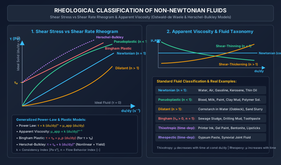
- 4.1 Shear Stress vs Shear Rate Rheogram & Apparent Viscosity Curves
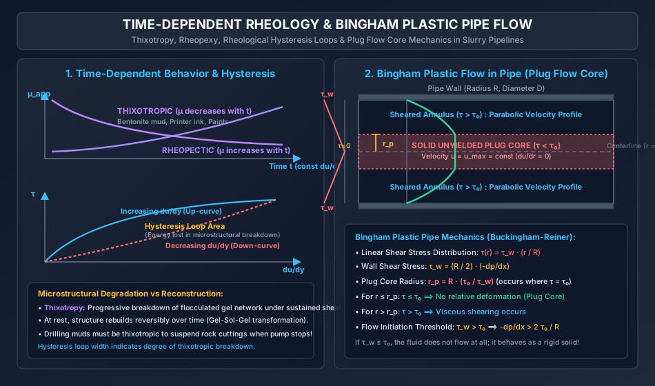
- 4.2 Time-Dependent Rheology & Bingham Plastic Pipe Flow (Plug Flow Core)
- 5. Comprehensive Step-by-Step Mathematical Derivations
- 5.1 Mechanics of Bingham Plastic Pipe Flow (Buckingham-Reiner Equation)
- 5.2 Flow Rate of a Power-Law Fluid in a Circular Pipe
- 6. Three Fully Worked Unit-Checked Numerical Examples
- Example 1: Apparent Viscosity & Shear Stress of a Pseudoplastic Fluid
- Example 2: Bingham Plastic Pipe Flow & Plug Core Radius
- Example 3: Pulling Force on Plate with Herschel-Bulkley Fluid Layer
- 7. Common Engineering Pitfalls & Examination Traps
- 8. Real-World Case Studies & Forensic Analysis
- Industrial Failure: Pipeline Blockage during Dredging Slurry Transport
- 9. Competitive Examination Practice Problems
- Problem 1 (GATE CE - 1 Mark)
- Problem 2 (UPSC ESE Paper-II - 2 Marks)
- Problem 3 (SSC JE - 1 Mark)
- Problem 4 (State PSC AE - 2 Marks)
- Problem 5 (RRB JE - 1 Mark)
- 10. Cross-Subject Synthesis & Advanced Fluid Couplings
- 11. Standard Reference Textbooks & Official Code Specifications
- 12. Comprehensive Summary, Formula Cheatsheet & Key Takeaways
1. Topic Metadata & Syllabus Mapping
| Attribute | Specification |
|---|---|
| Module / Topic ID | FM-01-02 |
| Subject | Fluid Mechanics & Hydraulic Machinery |
| Chapter | 01: Fluid Properties & Rheology |
| Topic Title | Rheological Classification and Behavior of Non-Newtonian Fluids |
| Primary Reference Standards | Ostwald-de Waele Model, Herschel-Bulkley Model, Bingham Plastic Model, Frank M. White (Fluid Mechanics), Bird, Stewart & Lightfoot (Transport Phenomena), Modi & Seth |
| Target Competitive Examinations | GATE CE, UPSC ESE (Paper-II), SSC JE, State PSC AE/JE, RRB JE |
| Examination Weightage | GATE (1 to 2 Marks), UPSC ESE (4 to 8 Marks prelims/mains), SSC JE (1 to 2 Marks), State AE/JE (2 Marks) |
| Prerequisites | FM-01-01 (Fluid Properties & Newton's Law of Viscosity) |
2. Executive Summary & Core Engineering Concepts
In engineering fluid mechanics, rheology is the science of the deformation and flow of matter. While simple fluids such as water, air, gasoline, and light lubricating oils obey Newton's Law of Viscosity () with a constant dynamic viscosity independent of the shear rate or duration of shear, a broad spectrum of engineering fluids—including drilling muds, sewage sludge, fresh concrete mixes, paints, blood, polymer melts, and clay suspensions—display non-linear or time-dependent stress-strain rate relationships. These substances are termed Non-Newtonian Fluids.
Non-Newtonian fluids are broadly categorized into three distinct classes:
- Time-Independent Fluids: Fluids where the shear stress at any point is a function solely of the instantaneous rate of shear strain (), described by the generalized Ostwald-de Waele Power-Law Model or the Herschel-Bulkley Yield-Power Law Model:
- Pseudoplastic (Shear-Thinning) Fluids (): Apparent viscosity decreases monotonically as shear rate increases (e.g., blood, milk, paint, polymeric solutions).
- Dilatant (Shear-Thickening) Fluids (): Apparent viscosity increases as shear rate increases (e.g., cornstarch suspensions / oobleck, concentrated wet sand).
- Bingham Plastics / Ideal Plastics (): Resist deformation as a rigid solid until an applied yield stress is exceeded, after which they flow linearly (e.g., sewage sludge, toothpaste, drilling mud).
- Herschel-Bulkley Fluids (): Possess both a yield stress and non-linear shear-thinning post-yield behavior (e.g., fresh concrete, heavy muds, greases).
- Time-Dependent Fluids: Fluids whose apparent viscosity changes with the duration of applied shearing:
- Thixotropic Fluids: Apparent viscosity decreases with time under sustained shear rate (e.g., bentonite drilling muds, printer inks, gel paints).
- Rheopectic Fluids: Apparent viscosity increases with time under sustained shear rate (e.g., gypsum paste, synovial fluid).
- Viscoelastic Fluids: Substances possessing both viscous fluid dissipation and elastic solid strain recovery (e.g., silly putty, liquid polymers exhibiting the Weissenberg rod-climbing effect).
3. Comprehensive Technical Principles & Mechanics
3.1 The Generalized Power-Law Model (Ostwald-de Waele)
For time-independent non-Newtonian fluids without an initial yield stress, the constitutive relation is expressed by the Ostwald-de Waele power-law equation:
Where:
- = Shear stress ( or ).
- = Rate of shear strain / velocity gradient ().
- = Flow Consistency Index, having dimensions and SI units .
- = Flow Behavior Index (dimensionless).
Concept of Apparent Viscosity ():
To maintain analogy with Newton's law (), we define the apparent viscosity:
+-----------------------------------------------------------------------------------+
| FLOW BEHAVIOR INDEX CLASSIFICATION:                                               |
|                                                                                   |
| 1. n = 1: NEWTONIAN FLUID                                                         |
|    - mu_app = k * (du/dy)^0 = k = mu = constant                                   |
|    - Shear stress is directly proportional to shear rate.                         |
|                                                                                   |
| 2. n < 1: PSEUDOPLASTIC (SHEAR-THINNING) FLUID                                    |
|    - Exponent (n - 1) is negative.                                                |
|    - As shear rate du/dy increases, mu_app DECREASES!                             |
|    - Microscopic mechanism: Randomly oriented polymer chains or elongated         |
|      molecules align with the streamlines, reducing hydraulic resistance.        |
|                                                                                   |
| 3. n > 1: DILATANT (SHEAR-THICKENING) FLUID                                       |
|    - Exponent (n - 1) is positive.                                                |
|    - As shear rate du/dy increases, mu_app INCREASES!                             |
|    - Microscopic mechanism: Closely packed solid particles dilate under shear;   |
|      interstitial liquid is drawn into expanding voids, increasing direct         |
|      interparticle contact friction.                                              |
+-----------------------------------------------------------------------------------+
3.2 Yield Stress Fluids: Bingham Plastic & Herschel-Bulkley Models
Certain materials behave as rigid solids until the applied shear stress exceeds a critical threshold known as the yield stress ().
1. Bingham Plastic Model:
Where:
- = Yield stress ().
- = Plastic viscosity (or Bingham viscosity) ().
- The apparent viscosity is: As , . As , .
2. Herschel-Bulkley (Yield Power-Law) Model:
Generalizes both the Bingham plastic and power-law models:
- If and : Reduces to Newtonian fluid ().
- If and : Reduces to Power-law fluid.
- If and : Reduces to Bingham plastic ().
- If and : Yield-pseudoplastic fluid (e.g., fresh concrete slurries, high-performance greases).
3.3 Time-Dependent Rheology: Thixotropy vs Rheopexy
In complex colloidal suspensions and emulsions, internal microstructures undergo physical aggregation or breakdown over time under steady shear:
                  TIME-DEPENDENT RHEOLOGY TAXONOMY

     Apparent Viscosity (μ_app) at CONSTANT Shear Rate (du/dy = const)

        μ_app ^
              |  \                                / Rheopectic (Structure Building)
              |   \  Thixotropic (Breakdown)     /   - Gypsum paste
              |    \                            /    - Synovial fluid
              |     \                          /
              |      +------------------------+---- Newtonian / Time-Independent
              |
              +-------------------------------------> Time (t)
- Thixotropic Fluids:
- Apparent viscosity decreases continuously with time when subjected to a constant shear rate:
- Under rest, the fluid rebuilds its gel structure through reversible Brownian flocculation.
- Civil Engineering Importance: Bentonite clay suspension used in diaphragm walls and well-drilling muds must be thixotropic. When drilling ceases, the mud rapidly thickens into a gel to hold rock cuttings in suspension, preventing drill string jamming. When pumping resumes, shear thins the mud instantly.
- Rheopectic Fluids (Anti-Thixotropic):
- Apparent viscosity increases continuously with time under sustained agitation:
- Example: Gypsum pastes, ammonium silicate suspensions, certain specialized printing lubricants.
4. Detailed Technical Diagrams & Visual Models
4.1 Shear Stress vs Shear Rate Rheogram & Apparent Viscosity Curves
The following hand-coded engineering diagram displays the comprehensive rheological classification of all fluid types on a vs rheogram, alongside the corresponding apparent viscosity curves demonstrating shear-thinning and shear-thickening behavior.
4.2 Time-Dependent Rheology & Bingham Plastic Pipe Flow (Plug Flow Core)
The following diagram illustrates the microscopic mechanism of thixotropic breakdown, the characteristic rheological hysteresis loop, and the velocity and shear stress profiles of a Bingham plastic flowing inside a circular pipe, highlighting the central unyielded solid plug core ().
5. Comprehensive Step-by-Step Mathematical Derivations
5.1 Mechanics of Bingham Plastic Pipe Flow (Buckingham-Reiner Equation)
Consider the steady, fully developed laminar flow of a Bingham plastic through a horizontal circular pipe of radius and length driven by an axial pressure drop .
-
Shear Stress Distribution across Pipe Cross-Section: Applying force equilibrium on a coaxial cylindrical fluid element of radius and length :
At the pipe wall ():
Crucial Property: The shear stress varies linearly from zero at the pipe centerline () to a maximum value at the pipe wall, regardless of the fluid's rheological model!
-
Condition for Flow Initiation: Flow can occur only if the wall shear stress exceeds the fluid yield stress:
If , the fluid remains a stationary rigid plug.
-
Plug Flow Core Formation (): Within the central region of the pipe where , the shear stress is insufficient to induce viscous yielding. The radius of the unyielded solid cylindrical plug core () is found where :
Inside this core ():
-
Velocity Distribution in the Sheared Annular Zone (): In this region, . The Bingham constitutive relation in pipe coordinates (where ) is:
Integrating with no-slip boundary condition at the pipe wall ():
-
Maximum / Plug Core Velocity ( at ): Substitute into the velocity equation:
-
Buckingham-Reiner Volumetric Flow Rate Equation: Integrating yields the celebrated Buckingham-Reiner Equation:
- When (Newtonian fluid), this reduces exactly to the Hagen-Poiseuille equation: .
5.2 Flow Rate of a Power-Law Fluid in a Circular Pipe
For an Ostwald-de Waele fluid ():
Integrating from to with :
The centerline maximum velocity:
Integrating for the volumetric flow rate :
- If and : (Hagen-Poiseuille formula).
6. Three Fully Worked Unit-Checked Numerical Examples
Example 1: Apparent Viscosity & Shear Stress of a Pseudoplastic Fluid
Problem Statement:
A polymeric drilling additive exhibits shear-thinning (pseudoplastic) behavior obeying the Ostwald-de Waele power-law model with flow consistency index and flow behavior index .
- Derive the mathematical expression for apparent viscosity .
- Calculate the shear stress and apparent viscosity at shear strain rates , , and .
- Discuss how the apparent viscosity changes over two orders of magnitude in shear rate.
Step-by-Step Solution:
Step 1: Formulations Power-law shear stress:
Apparent viscosity:
Step 2: Evaluations at Specified Shear Rates
-
At :
-
At :
-
At :
Step 3: Engineering Analysis As the shear rate increases from to (a 100-fold increase), the apparent viscosity drops from to (an reduction). This demonstrates the pronounced shear-thinning property crucial in industrial pumping where high pipeline shear rates reduce required pumping head.
Example 2: Bingham Plastic Pipe Flow & Plug Core Radius
Problem Statement:
Digested sewage sludge behaving as a Bingham plastic with yield stress and plastic viscosity is pumped through a horizontal circular cast-iron pipeline of diameter (). The measured shear stress at the pipe wall is .
- Verify whether flow occurs.
- Determine the radius of the unsheared central solid plug core and the ratio .
- Calculate the axial pressure gradient in .
- Calculate the velocity gradient (shear rate) at the pipe wall.
Step-by-Step Solution:
Step 1: Flow Verification
Since wall shear stress exceeds the threshold yield stress, the fluid yields adjacent to the pipe walls and flow takes place.
Step 2: Plug Core Radius The shear stress varies linearly across the pipe radius: . The boundary of the plug core occurs where :
Plug-to-pipe radius ratio:
Step 3: Axial Pressure Gradient From cross-sectional equilibrium:
Step 4: Shear Rate at the Pipe Wall For , the Bingham plastic constitutive equation is:
At the wall ():
Example 3: Pulling Force on Plate with Herschel-Bulkley Fluid Layer
Problem Statement:
A flat thin plate of surface area is pulled horizontally at a steady velocity over a stationary flat surface. The gap between the plate and the surface has a uniform thickness and is filled with a Herschel-Bulkley fluid characterized by:
- Yield stress:
- Consistency index:
- Flow behavior index:
- Calculate the shear rate across the gap.
- Determine the shear stress and apparent viscosity .
- Determine the required horizontal pulling force .
- Compare this force with that required for a Newtonian fluid of viscosity .
Step-by-Step Solution:
Step 1: Shear Rate Assuming a linear velocity distribution across the narrow gap ():
Step 2: Shear Stress and Apparent Viscosity Herschel-Bulkley equation:
Apparent viscosity:
Step 3: Required Pulling Force
Step 4: Comparison with Newtonian Fluid ()
The Herschel-Bulkley fluid requires only vs for the Newtonian fluid (an force reduction) due to its strong shear-thinning post-yield response ().
7. Common Engineering Pitfalls & Examination Traps
| Pitfall / Exam Trap | Erroneous Concept | Correct Physical & Code Principle |
|---|---|---|
| Trap 1: Confusing Pseudoplasticity with Thixotropy | Treating shear-thinning (pseudoplastic) and thixotropic fluids as interchangeable. | Pseudoplasticity is time-independent: depends only on the magnitude of shear rate . Thixotropy is time-dependent: decreases with the duration of applied shearing at constant . |
| Trap 2: Assuming Non-Zero Velocity Gradient Inside Plug Core | Applying viscous shear equations across the entire pipe radius for Bingham fluids. | Inside the plug core (), . Hence, . The fluid does not deform; it moves as a solid translatory block at uniform velocity . |
| Trap 3: Units of Consistency Index | Assuming always has units of . | The unit of depends strictly on : . Only when does become . For , . |
| Trap 4: Forgetting that Pipe Shear Stress is Independent of Fluid Type | Assuming non-Newtonian fluids have non-linear shear stress profiles in pipes. | The shear stress distribution is derived purely from static force equilibrium. It is strictly linear for ALL fluids (Newtonian, Bingham, Pseudoplastic, Dilatant, Turbulent). Only the velocity profile changes! |
| Trap 5: Misidentifying Blood & Paint | Classifying blood or house paint as Bingham plastics. | Blood and latex house paint are classic Pseudoplastics (shear-thinning, ). Toothpaste and drilling mud are Bingham plastics (). |
8. Real-World Case Studies & Forensic Analysis
Industrial Failure: Pipeline Blockage during Dredging Slurry Transport
- Context: An environmental dredging project in a major Indian harbor pumped high-density silt-clay slurry through a offshore discharge pipeline ().
- The Failure: During a scheduled 2-hour maintenance shutdown of the slurry pumps, the flow was abruptly stopped. Upon pump restart, the pump developed its maximum rated discharge pressure of (), but zero flow could be initiated. The pipeline remained completely seized, forcing emergency divers and line cutting costing millions.
- Forensic Rheological Analysis:
- The dredged bentonitic silt slurry was thixotropic with a rest-state yield stress that grew from during shearing to after 2 hours of quiescent gelation.
- To initiate flow, the required wall shear stress was .
- The required restart pressure drop was:
- The pumps could only generate , creating an irrecoverable hydraulic deadlock.
- Engineering Remediation: Installation of water-flush bypass systems prior to shutdowns and continuous low-frequency pressure pulsing to disrupt thixotropic gel lattice formation.
9. Competitive Examination Practice Problems
Problem 1 (GATE CE - 1 Mark)
A fluid whose apparent viscosity decreases with an increase in velocity gradient is classified as:
- (A) Dilatant fluid
- (B) Pseudoplastic fluid
- (C) Bingham plastic
- (D) Rheopectic fluid
Correct Answer: (B)
Step-by-Step Explanation:
For a pseudoplastic (shear-thinning) fluid, the flow behavior index is . Apparent viscosity decreases as increases.
Problem 2 (UPSC ESE Paper-II - 2 Marks)
Match List-I (Fluids) with List-II (Rheological Classification) and select the correct answer:
- A. Sewage sludge 1. Dilatant
- B. Blood 2. Bingham Plastic
- C. Concentrated sugar/cornstarch suspension 3. Pseudoplastic
- D. Bentonite slurry at rest 4. Thixotropic
Codes (A - B - C - D):
- (A) 2 - 3 - 1 - 4
- (B) 3 - 2 - 1 - 4
- (C) 2 - 1 - 3 - 4
- (D) 4 - 3 - 1 - 2
Correct Answer: (A)
Step-by-Step Explanation:
- Sewage sludge requires an initial yield stress and flows linearly Bingham Plastic (2).
- Blood consists of deformable red blood cells that align under shear Pseudoplastic (3).
- Cornstarch in water thickens violently under shear Dilatant (1).
- Bentonite clay mud thickens over time at rest Thixotropic (4).
Problem 3 (SSC JE - 1 Mark)
Toothpaste is an engineering example of:
- (A) Newtonian fluid
- (B) Bingham plastic
- (C) Dilatant fluid
- (D) Ideal fluid
Correct Answer: (B)
Step-by-Step Explanation:
Toothpaste does not flow out of the tube under gravity alone (it acts as a solid because ). When squeezed, the yield stress is exceeded and it flows easily Bingham plastic.
Problem 4 (State PSC AE - 2 Marks)
In laminar flow of a Bingham plastic through a pipe of radius , the shear stress at radius is:
- (A) Zero everywhere
- (B) Constant across the cross-section
- (C) Directly proportional to the radial distance
- (D) Proportional to
Correct Answer: (C)
Step-by-Step Explanation:
From static force balance on a fluid cylinder of radius :
The shear stress varies strictly linearly with radius , completely independent of the fluid's rheological model.
Problem 5 (RRB JE - 1 Mark)
A fluid for which the apparent viscosity increases with the duration of applied shear stress at a constant shear rate is called:
- (A) Thixotropic
- (B) Rheopectic
- (C) Pseudoplastic
- (D) Dilatant
Correct Answer: (B)
Step-by-Step Explanation:
A time-dependent fluid whose viscosity increases with time under sustained shearing is defined as rheopectic. (If it decreases with time, it is thixotropic).
10. Cross-Subject Synthesis & Advanced Fluid Couplings
                             CROSS-DISCIPLINARY SYNTHESIS

    Non-Newtonian Fluid Rheology (FM-01-02)
    - Yield Stress tau_0 & Apparent Viscosity mu_app(gamma)
    - Herschel-Bulkley Model (tau = tau_0 + k gamma^n)
                         |
                         v
    Concrete Technology (SUB-04) & Geotechnical Engineering (SUB-09)
    - Self-Compacting Concrete (SCC) Rheology: Slump flow governed by tau_0; V-funnel by mu_app
    - Bentonite Slurry Trench Stability: Hydrostatic support + Filter cake gelation (thixotropy)
                         |
                         v
    Environmental Engineering (SUB-10)
    - Sewage Slurry Pipeline Hydraulics (Head loss via Buckingham-Reiner equation)
    - Sludge Dewatering in Centrifuges & Filter Presses
11. Standard Reference Textbooks & Official Code Specifications
- R. Byron Bird, Warren E. Stewart, Edwin N. Lightfoot: Transport Phenomena, 2nd Edition, John Wiley & Sons, Chapter 1: Viscosity and the Mechanisms of Momentum Transport.
- Frank M. White: Fluid Mechanics, 8th Edition, McGraw-Hill, Chapter 1: Non-Newtonian Fluids.
- P.N. Modi & S.M. Seth: Hydraulics and Fluid Mechanics Including Hydraulic Machines, Standard Book House, New Delhi, Chapter 1: Properties of Fluids.
- H.A. Barnes, J.F. Hutton, K. Walters: An Introduction to Rheology, Elsevier Science Publishers.
- IS 4987: Recommendations for Design and Installation of Flow Measurement Devices, BIS, New Delhi.
12. Comprehensive Summary, Formula Cheatsheet & Key Takeaways
===================================================================================================
                       NON-NEWTONIAN FLUID RHEOLOGY CHEATSHEET
===================================================================================================
1. Ostwald-de Waele Power-Law Model (tau_0 = 0):
   - Constitutive Law:    tau = k * (du/dy)^n
   - Apparent Viscosity:  mu_app = k * (du/dy)^(n - 1)
   - Newtonian:           n = 1  ==> mu_app = const = mu (Water, Air, Oil)
   - Pseudoplastic:       n < 1  ==> mu_app DECREASES with shear rate (Blood, Paint, Mud)
   - Dilatant:            n > 1  ==> mu_app INCREASES with shear rate (Oobleck, Sand slurry)

2. Yield Stress Models:
   - Bingham Plastic:     tau = tau_0 + mu_p * (du/dy)       (for tau > tau_0)
                          mu_app = mu_p + tau_0 / (du/dy)
   - Herschel-Bulkley:    tau = tau_0 + k * (du/dy)^n        (for tau > tau_0)

3. Time-Dependent Behavior (const du/dy):
   - Thixotropic:         (d mu_app / dt) < 0  ==> Viscosity DROPS with time (Bentonite, Inks)
   - Rheopectic:          (d mu_app / dt) > 0  ==> Viscosity RISES with time (Gypsum paste)

4. Bingham Pipe Flow (Buckingham-Reiner):
   - Shear Stress:        tau(r) = tau_w * (r / R)           (Linear everywhere)
   - Wall Shear Stress:   tau_w = (R / 2) * (-dp/dx)
   - Flow Condition:      tau_w > tau_0  ==> -dp/dx > 2 tau_0 / R
   - Plug Core Radius:    r_p = R * (tau_0 / tau_w)          (Solid plug, du/dr = 0)
   - Flow Rate:           Q = [pi R^4 dp] / [8 mu_p L] * [1 - (4/3)(tau_0/tau_w) + (1/3)(tau_0/tau_w)^4]
===================================================================================================