Dimensional Homogeneity, Rayleigh's Method & Buckingham -Theorem
In this chapter (2 topics)
On this page
- 1. Topic Metadata Table
- 2. Executive Summary
- 3. Fundamental Dimensions (MLT vs FLT) & Derived Physical Properties
- 3.1 The MLT and FLT Systems of Dimensions
- 3.2 Master Dimensional Table of Fluid Parameters
- 4. Principle of Dimensional Homogeneity (Fourier's Principle)
- 4.1 Statement of the Principle
- 4.2 Diagnostic Utility
- 5. Rayleigh's Indeterminate Power-Law Method
- 5.1 Formulation
- 5.2 Solution Algorithm
- 5.3 Limitations of Rayleigh's Method
- 6. Buckingham π-Theorem & Dimensional Matrix Rank Criterion (k = n - m)
- 6.1 Statement of the Theorem
- 6.2 The Matrix Rank Criterion (Van Driest's Generalization)
- 7. Rules Governing Selection of Repeating Variables
- The Five Mandatory Selection Rules:
- 8. Visual Diagrams & Methodological Schematics
- 8.1 Buckingham π-Theorem Step-by-Step Flowchart
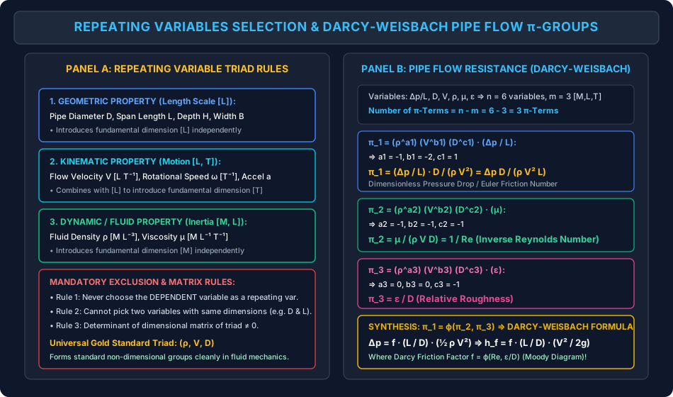
- 8.2 Repeating Variables Selection & Pipe Flow π-Groups Breakdown
- 9. Step-by-Step Numerical Problems with Complete Calculations
- Problem 1: Pipe Resistance & Derivation of Darcy-Weisbach Equation
- Problem 2: Drag Force on a Submerged Sphere — Rayleigh's Method vs Stokes' Law
- Problem 3: Turbomachine Power Coefficient & Dynamic Scale Prediction
- 10. High-Yield Exam Pitfalls, Traps & Shortcuts
- 11. Multi-Exam Question Bank (GATE, ESE, SSC JE, State AE, RRB JE)
- Question 1 (GATE CE — Multiple Choice Question)
- Question 2 (UPSC ESE Paper-II)
- Question 3 (SSC JE)
- Question 4 (State PSC AE)
- Question 5 (RRB JE)
- 12. Comprehensive Summary, Formula Cheatsheet & Academic References
- Master Formula Cheatsheet
- Academic References & Standard Source Texts
1. Topic Metadata Table
| Field | Detail |
|---|---|
| Subject | Fluid Mechanics & Hydraulic Machinery (Subject 07) |
| Chapter | Chapter 05: Dimensional Analysis & Model Similitude |
| Topic Code | FM-05-01 |
| Topic Title | Dimensional Homogeneity, Rayleigh's Indeterminate Power-Law Method, Buckingham -Theorem, Dimensional Matrix Rank Criterion (), and Repeating Variables Selection Rules |
| Prerequisites | High School Physics (Units & Dimensions), Matrix Algebra (Rank & Determinants), FM-01-01 to FM-01-04 (Fluid Properties: ) |
| Target Examinations | GATE CE, UPSC ESE (Paper-II), SSC JE, State PSC AE/JE, RRB JE |
| Knowledge Level | Fundamental Dimensional Matrix Theory to Applied Hydraulic Flow Grouping |
| IS / ISO / Standard Codes | IS 1192 (Velocity measurement in open channels), ISO 31-3 (Quantities and units - Mechanics), ASTM E380 (Standard Practice for Use of the International System of Units) |
| Key Formulae | , , , , , |
2. Executive Summary
Dimensional analysis is a powerful mathematical technique that condenses complex multi-variable physical phenomena into compact, generalized equations governed by dimensionless groups. By exploiting the fundamental requirement that physical laws must remain valid irrespective of the system of measurement units chosen (The Principle of Dimensional Homogeneity), dimensional analysis reduces the number of experimental parameters, guides scale-model testing, eliminates dimensional artifacts, and uncovers the underlying similitude laws governing engineering hydraulics.
Two systematic analytical frameworks exist:
- Rayleigh's Method of Dimensional Analysis:
- Expresses the dependent variable as an exponential product of independent parameters:
- By equating exponents of the primary dimensions ( or ) across both sides of the equation, a system of simultaneous linear equations is solved.
- While elegant and intuitive for simple systems involving 3 or 4 variables, Rayleigh's method becomes algebraically cumbersome and indeterminate when the number of variables exceeds the number of primary dimensions by more than two.
- The Buckingham -Theorem (Edgar Buckingham, 1914):
- The cornerstone of modern dimensional analysis. It states: If a physical process involves dimensional variables (both dependent and independent) containing fundamental dimensions (), the entire phenomenon can be grouped into independent dimensionless -terms:
- More rigorously, represents the Rank of the Dimensional Matrix formed by the variables. If the matrix rank , the number of dimensionless terms is .
Rules Governing Selection of Repeating Variables: To form the -groups, repeating variables must be selected that appear in every -term. Successful execution demands strict adherence to five inviolable rules:
- The number of repeating variables chosen must equal (the rank of the dimensional matrix, typically ).
- The repeating variables must collectively encompass all fundamental dimensions ().
- The repeating variables must not form a dimensionless group among themselves (the determinant of their dimensional sub-matrix must be non-zero: ).
- The dependent variable must NEVER be chosen as a repeating variable.
- Standard civil/mechanical engineering convention mandates selecting one variable from each of three distinct physical classes:
- One Geometric Property: Linear dimension (Pipe diameter , length , depth ).
- One Kinematic / Flow Property: Motion parameter (Velocity , angular speed , acceleration ).
- One Fluid Dynamic / Inertial Property: Fluid property (Density , dynamic viscosity , surface tension ).
The universal "Gold Standard" repeating triad in fluid mechanics is . Applying Buckingham -theorem with this triad to closed-conduit pipe resistance yields the celebrated Darcy-Weisbach Equation (), where the dimensionless friction factor emerges organically as a function of the Reynolds Number () and Relative Roughness ().
3. Fundamental Dimensions ( vs ) & Derived Physical Properties
In physical continuum mechanics, all measurable parameters are formulated in terms of a small set of primary, mutually independent base dimensions:
3.1 The and Systems of Dimensions
- System (Mass-Length-Time): Standard absolute system where Mass , Length , and Time are primary base units.
- System (Force-Length-Time): Gravitational / Engineering system where Force , Length , and Time are primary base units.
The two systems are interconnected through Newton's second law ():
3.2 Master Dimensional Table of Fluid Parameters
| Parameter | Symbol | SI Unit | Dimension | Dimension |
|---|---|---|---|---|
| Length / Diameter / Roughness | ||||
| Area | ||||
| Volume | ||||
| Velocity (Linear) | ||||
| Acceleration / Gravity | ||||
| Angular Velocity / Rotational Speed | ||||
| Volumetric Discharge | ||||
| Mass Flow Rate | ||||
| Density | ||||
| Specific Weight | ||||
| Force / Thrust / Drag / Lift | ||||
| Pressure / Stress / Elastic Modulus | () | |||
| Dynamic Viscosity | ||||
| Kinematic Viscosity | ||||
| Surface Tension | ||||
| Work / Energy / Torque | ||||
| Power |
4. Principle of Dimensional Homogeneity (Fourier's Principle)
4.1 Statement of the Principle
The Principle of Dimensional Homogeneity states:
Any physically meaningful equation expressing a relationship between physical quantities must have the same fundamental dimensions in every separate additive term on both sides of the equation.
Mathematically, if an equation is of the form:
then:
Furthermore:
- Arguments of all transcendental functions (trigonometric , exponential , logarithmic ) must be strictly dimensionless ().
- Pure numerical constants (e.g., ) are dimensionless.
- If an equation is dimensionally homogeneous, its validity is independent of the system of units employed (it holds equally in SI, BG, or English Engineering units without requiring conversion factors).
4.2 Diagnostic Utility
Dimensional homogeneity serves as a rapid, infallible error check:
- If an analytical derivation yields an equation with mismatched dimensions (e.g., adding to ), the derivation is categorically flawed.
- However, dimensional homogeneity is a necessary condition, not a sufficient condition: an equation can be dimensionally consistent yet physically incorrect due to missing dimensionless numerical factors (such as a factor of or ).
5. Rayleigh's Indeterminate Power-Law Method
5.1 Formulation
Lord Rayleigh's method assumes that the dependent variable is related to independent variables through a direct power-law product:
where is a dimensionless numerical proportionality constant, and are unknown constant exponents.
5.2 Solution Algorithm
- Substitute the dimensions of each variable in into the power-law equation.
- Group and equate the exponents of , , and separately on the left-hand and right-hand sides, generating simultaneous linear algebraic equations.
- If the number of independent variables is , the three exponents are determined uniquely.
- If the number of independent variables exceeds , solve for of the exponents in terms of the remaining undetermined exponents.
- Re-substitute the expressions into the original equation and collect terms with identical exponents into dimensionless groups.
5.3 Limitations of Rayleigh's Method
- When the number of variables exceeds or , solving the system of indeterminate equations becomes convoluted and prone to algebraic errors.
- Rayleigh's method provides no formal criteria for choosing which exponents to eliminate or how to structure the resulting non-dimensional groups.
- For systems involving variables, the Buckingham -Theorem provides a far superior, algorithmic matrix-based procedure.
6. Buckingham -Theorem & Dimensional Matrix Rank Criterion ()
6.1 Statement of the Theorem
Let a physical phenomenon depend on physical variables :
If these variables contain primary fundamental dimensions (), then the equation can be reformulated in terms of independent dimensionless groups (-terms):
or, expressing one dimensionless group explicitly as a function of the others:
6.2 The Matrix Rank Criterion (Van Driest's Generalization)
In classical textbooks, is casually stated as the number of fundamental dimensions (usually for ). However, this is an oversimplification that fails when certain dimensions are absent or coupled.
The mathematically rigorous statement is:
is equal to the RANK of the Dimensional Matrix formed by the physical variables.
The Dimensional Matrix is an matrix whose rows represent the primary dimensions () and whose columns represent the exponent powers of each variable:
- The rank is the size of the largest square sub-matrix with a non-zero determinant.
- Usually, for problems involving .
- Special Cases ():
- If mass is completely absent from all variables (kinematic problems involving only and , such as surface wave propagation or vortex kinematics), the -row is entirely zero .
- In such cases, the number of -terms is:
7. Rules Governing Selection of Repeating Variables
To formulate the dimensionless -groups, an engineer must choose variables from the available parameters to serve as Repeating Variables that appear in every -term. The remaining non-repeating variables are combined with the repeating set one at a time.
Total Variables: n
+-----------------------+-----------------------------+
| Repeating Set: m      | Non-Repeating Set: (n - m)  |
| (D, V, rho)           | (Delta p, mu, epsilon, ...) |
+-----------------------+-----------------------------+
          |                            |
          +-----------> [ x 1 ] <------+
                          |
                          v
                 pi_i = (Repeating)^exponents * (Non-Repeating)
The Five Mandatory Selection Rules:
- Rule 1: Number of Repeating Variables = (Rank )
- For fluid dynamics problems involving mass, length, and time, exactly repeating variables must be selected.
- Rule 2: Collective Dimensional Completeness
- The selected repeating variables must collectively contain all fundamental dimensions ().
- Violation Example: Selecting fails because none contains Mass .
- Rule 3: Mutual Dimensional Independence ()
- The repeating variables must not form a dimensionless group among themselves.
- Mathematically: The determinant formed by the dimensional matrix of the repeating variables must be non-zero:
- Violation Example: Choosing fails because is already dimensionless ().
- Rule 4: Dependent Variable Exclusion
- The primary dependent variable being solved for (e.g., Drag force , pressure drop , power ) must NEVER be chosen as a repeating variable.
- Keeping the dependent variable isolated ensures that it appears in only one -term (), allowing the final equation to be solved explicitly: .
- Rule 5: The Three-Category Engineering Heuristic
- To guarantee physical clarity and satisfy Rules 1–3 automatically, select:
- One Geometric Property: Linear dimension characterizing size ().
- One Kinematic Property: Motion parameter characterizing flow rate ().
- One Fluid Dynamic / Inertial Property: Fluid property characterizing mass/forces ().
- The Universal Standard Triad: This triad satisfies all matrix independence conditions and guarantees that standard engineering dimensionless groups () emerge cleanly.
- To guarantee physical clarity and satisfy Rules 1–3 automatically, select:
8. Visual Diagrams & Methodological Schematics
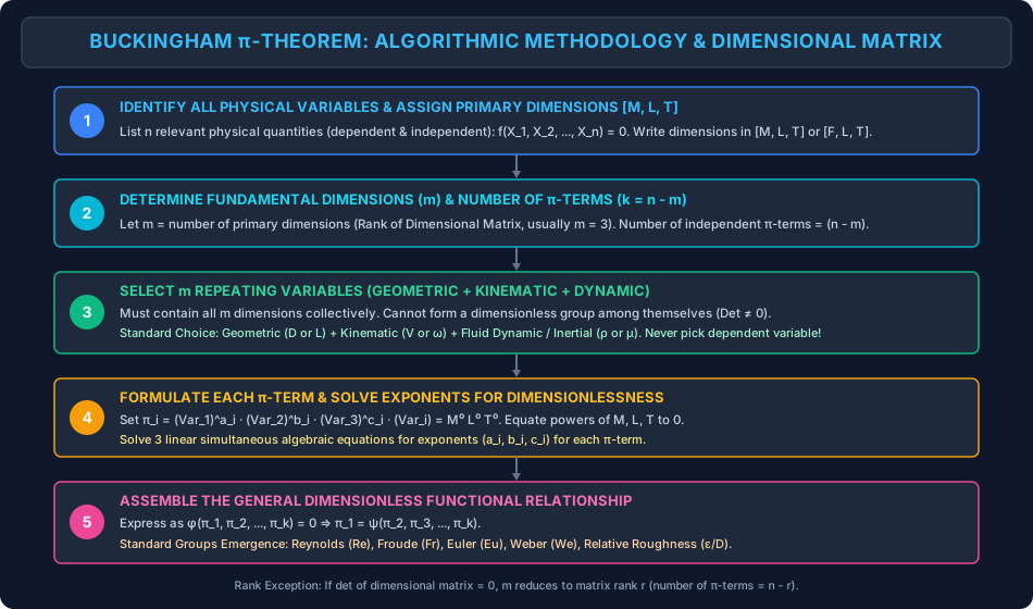
8.1 Buckingham -Theorem Step-by-Step Flowchart
The flowchart below details the systematic, five-step algorithmic procedure for executing Buckingham dimensional analysis, highlighting the rank verification gate.
8.2 Repeating Variables Selection & Pipe Flow -Groups Breakdown
The multi-panel diagram below illustrates the geometric-kinematic-dynamic triad selection rules and details the complete derivation of the Darcy-Weisbach pipe friction equation from first principles.
9. Step-by-Step Numerical Problems with Complete Calculations
Problem 1: Pipe Resistance & Derivation of Darcy-Weisbach Equation
Problem Statement: The pressure drop per unit length of a pipeline carrying steady incompressible fluid depends on:
- Mean flow velocity ,
- Pipe internal diameter ,
- Fluid density ,
- Fluid dynamic viscosity ,
- Equivalent sand-grain surface roughness height .
Execute the following:
- Using Buckingham's -theorem, derive the general dimensionless functional relationship, proving that the Darcy-Weisbach friction formula is dimensionally exact: where .
- Numerical Evaluation: Water () flows through a commercial steel pipe () of length with wall roughness at a velocity .
- Compute the Reynolds number and relative roughness .
- If the Darcy friction factor is , calculate the head loss in meters of water and the pressure drop in ().
Solution & Step-by-Step Calculation:
Step 1: Variables and Dimensional Matrix Total physical variables :
- Dependent variable:
- Independent variables: , , , , .
Fundamental dimensions: (). Number of independent -terms:
Select repeating variables: (Dynamic, Kinematic, Geometric triad). Check determinant of repeating variables dimensional matrix:
Step 2: Formulate (Pressure Drop per Unit Length)
Equating exponents:
- For :
- For :
- For :
Therefore:
Step 3: Formulate (Viscosity Group / Reynolds Number)
Equating exponents:
- For :
- For :
- For :
Therefore:
Step 4: Formulate (Surface Roughness Group)
By inspection, since and both possess dimension and zero mass/time:
Step 5: General Synthesis
Defining the Darcy friction factor :
Step 6: Numerical Calculation
- Reynolds number:
- Relative roughness:
- Head loss :
- Pressure drop :
Problem 2: Drag Force on a Submerged Sphere — Rayleigh's Method vs Stokes' Law
Problem Statement: The aerodynamic or hydrodynamic drag force acting on a smooth sphere moving through a fluid depends on:
- Sphere diameter ,
- Relative flow velocity ,
- Fluid density ,
- Fluid dynamic viscosity .
Execute the following:
- Use Rayleigh's exponential method to show that:
- Show how this general relationship yields the definition of the drag coefficient .
- For very low Reynolds numbers (, creeping Stokes flow), the drag force is known to be independent of fluid density . Prove that this condition forces the exponent of to be , yielding Stokes' Law:
- Numerical Check: A small glass sphere of diameter settles in glycerin () at terminal velocity .
- Verify that the flow is in the Stokes regime ().
- Compute the drag coefficient .
- Calculate the drag force in .
Solution & Step-by-Step Calculation:
Step 1: Rayleigh's Formulation
Dimensions:
Equating exponents:
- For :
- For :
- For :
Substitute exponents back into the formulation:
Step 2: Relation to Drag Coefficient Frontal projected area of the sphere: .
Step 3: Stokes Flow Independence of Density In creeping laminar flow (), inertial forces are negligible compared to viscous forces; hence, drag cannot depend on fluid density . From :
Substituting :
Hydrodynamic theory (George Gabriel Stokes, 1851) proves the exact constant is :
Step 4: Numerical Calculation
- Reynolds number: Since , flow is strictly in the creeping laminar Stokes regime!
- Drag coefficient :
- Drag force :
- Using Stokes' equation:
- Using standard formulation:
Problem 3: Turbomachine Power Coefficient & Dynamic Scale Prediction
Problem Statement: The shaft power required to operate a rotodynamic mixer/pump impeller depends on:
- Impeller diameter ,
- Rotational speed (),
- Fluid density ,
- Fluid dynamic viscosity ,
- Volumetric discharge .
Execute the following:
- Apply the Buckingham -theorem choosing repeating variables to derive the dimensionless Power Coefficient (), Flow Coefficient (), and Rotational Reynolds Number ():
- Numerical Scale Prediction:
- A model impeller with diameter rotating at () in water () consumes shaft power ().
- Determine the dimensionless power coefficient .
- A geometrically similar prototype impeller of diameter is designed to operate at () in a denser chemical solution with .
- Assuming dynamically similar conditions (identical ), calculate the shaft power required to drive the prototype impeller in .
Solution & Step-by-Step Calculation:
Step 1: Variables and Dimensions Variables : , , , , . (For fixed discharge ratio, ). Primary dimensions: (). Number of -terms: (or including ).
Repeating variables: . Check dimensions: , , .
Step 2: Formulate Power Coefficient
Equating exponents:
- For :
- For :
- For :
Therefore:
(Similarly: and ).
Step 3: Numerical Evaluation for Model Impeller
Compute Power Coefficient :
Step 4: Scale Prediction for Prototype Impeller
- (Geometric scale ratio )
For dynamic similarity, :
Compute components:
(Alternatively, by scaling ratio: ).
10. High-Yield Exam Pitfalls, Traps & Shortcuts
-
The Dependent Repeating Variable Trap (GATE CE):
- Trap: Choosing the dependent parameter (e.g., Drag force or pressure drop ) as one of the repeating variables.
- Truth: If the dependent parameter is chosen as repeating, it will appear in multiple -terms, resulting in an implicit transcendental equation that cannot be isolated as . Always keep the dependent parameter in the non-repeating set!
-
The "Dimensionless Triad" Trap (UPSC ESE):
- Trap: Selecting as repeating variables.
- Truth: , , . The term is already dimensionless! The determinant of their dimensional matrix is zero; they are not independent.
-
Counting Fundamental Dimensions: The Rank Exception:
- Trap: Automatically assuming because are listed in the textbook.
- Truth: Always verify that all 3 dimensions are present. In pure kinematics () or problems where force parameters cannot be decomposed independently, the matrix rank may be . Number of -terms is strictly .
-
Transcendental Arguments Must Be Dimensionless:
- Any function such as , , or requires that the internal arguments , , and be strictly dimensionless ().
-
Kinematic vs Dynamic Viscosity Dimensions:
- Dynamic viscosity : (or ).
- Kinematic viscosity : (No mass!).
11. Multi-Exam Question Bank (GATE, ESE, SSC JE, State AE, RRB JE)
Question 1 (GATE CE — Multiple Choice Question)
The variables involved in a hydraulic phenomenon are discharge , head , acceleration due to gravity , fluid density , dynamic viscosity , and width . If the fundamental dimensions are , the number of independent dimensionless groups (-terms) required to describe the phenomenon is:
- A) 2
- B) 3
- C) 4
- D) 5
Detailed Solution: List variables: . Total variables . Fundamental dimensions present: (in ), , . Thus . Rank of dimensional matrix . By Buckingham -theorem, number of -terms is:
Correct Answer: B
Question 2 (UPSC ESE Paper-II)
Which of the following combinations CANNOT be selected as repeating variables in Buckingham's -theorem for a fluid flow problem involving dimensions ?
- A) Velocity , Pipe diameter , Fluid density
- B) Length , Flow velocity , Dynamic viscosity
- C) Pipe diameter , Rotational speed , Flow velocity
- D) Discharge , Pipe diameter , Fluid density
Detailed Solution: In option C, , , and . Notice that:
The group is already dimensionless among themselves, violating the rule of mutual independence (). Furthermore, none of the three variables contains Mass . Correct Answer: C
Question 3 (SSC JE)
The dimensions of dynamic viscosity () in the system and the system are respectively:
- A) and
- B) and
- C) and
- D) and
Detailed Solution: Shear stress . In : . In : . Correct Answer: A
Question 4 (State PSC AE)
If an equation is dimensionally homogeneous:
- A) It must be physically correct in every aspect
- B) Every additive term must have the same dimensions, but it may still be physically incomplete or wrong by a numerical constant
- C) It is valid only in the SI system of units
- D) The number of variables must equal the number of primary dimensions
Detailed Solution: Dimensional homogeneity is a necessary but not sufficient condition for physical correctness. It ensures identical dimensions across terms, making the equation unit-independent, but cannot detect missing dimensionless coefficients. Correct Answer: B
Question 5 (RRB JE)
According to Rayleigh's method of dimensional analysis, the maximum number of independent variables that can be uniquely evaluated using three fundamental dimensions () without remaining indeterminate is:
- A) 2
- B) 3
- C) 4
- D) 5
Detailed Solution: Because three fundamental dimensions () provide exactly 3 independent linear equations, at most 3 independent variable exponents can be uniquely determined without requiring parametric groupings. Correct Answer: B
12. Comprehensive Summary, Formula Cheatsheet & Academic References
Master Formula Cheatsheet
Academic References & Standard Source Texts
- White, F. M. (2016). Fluid Mechanics (8th ed.). McGraw-Hill Education. Chapter 5: Dimensional Analysis and Similarity.
- Modi, P. N., & Seth, S. M. (2018). Hydraulics and Fluid Mechanics Including Hydraulics Machines (22nd ed.). Standard Book House, New Delhi. Chapter 12: Dimensional Analysis and Model Similitude.
- Streeter, V. L., Wylie, E. B., & Bedford, K. W. (1998). Fluid Mechanics (9th ed.). WCB/McGraw-Hill. Chapter 5: Dimensional Analysis and Dynamic Similitude.
- Rajput, R. K. (2020). A Textbook of Fluid Mechanics and Hydraulic Machines (7th ed.). S. Chand & Company Ltd. Chapter 12: Dimensional and Model Analysis.
- ISO 31-3: Quantities and Units - Part 3: Mechanics. International Organization for Standardization.