Model Similitude, Dimensionless Numbers & Distorted River Models
In this chapter (2 topics)
On this page
- 1. Topic Metadata Table
- 2. Executive Summary
- 3. Geometric, Kinematic & Dynamic Similitude
- 3.1 Geometric Similarity (Similarity of Shape)
- 3.2 Kinematic Similarity (Similarity of Motion)
- 3.3 Dynamic Similarity (Similarity of Forces)
- 4. The Five Primary Dimensionless Numbers & Force Ratios
- 4.1 Master Dimensionless Groups Table
- 5. Model Laws: Reynolds vs Froude Model Law Scale Derivations
- 5.1 Froude Model Law (Frm = Frp)
- 5.2 Reynolds Model Law (Rem = Rep)
- 6. Distorted Models in Civil Engineering: River, Estuary & Harbor Hydraulics
- 6.1 Undistorted vs Distorted Models Defined
- 6.2 Why Distortion is Essential for River and Harbor Models
- 6.3 Mathematical Scale Ratios for Distorted Froude Models
- 7. Scale Effects & Limitations of Hydraulic Scale Modeling
- Common Scale Effects in Civil Hydraulics:
- 8. Visual Diagrams & Hydraulic Schematics
- 8.1 Froude vs Reynolds Model Laws Comparison
- 8.2 Distorted River Model Similitude & Scale Ratios
- 9. Step-by-Step Numerical Problems with Complete Calculations
- Problem 1: Froude Model Law on Dam Spillway & Stilling Basin
- Problem 2: Reynolds Model Law — Submarine in Water Tunnel
- Problem 3: Distorted River Model — Scales, Discharge & Roughness Adaptation
- 10. High-Yield Exam Pitfalls, Traps & Shortcuts
- 11. Multi-Exam Question Bank (GATE, ESE, SSC JE, State AE, RRB JE)
- Question 1 (GATE CE — Multiple Choice Question)
- Question 2 (UPSC ESE Paper-II)
- Question 3 (SSC JE)
- Question 4 (State PSC AE)
- Question 5 (RRB JE)
- 12. Comprehensive Summary, Formula Cheatsheet & Academic References
- Master Formula Cheatsheet
- Academic References & Standard Source Texts
1. Topic Metadata Table
| Field | Detail |
|---|---|
| Subject | Fluid Mechanics & Hydraulic Machinery (Subject 07) |
| Chapter | Chapter 05: Dimensional Analysis & Model Similitude |
| Topic Code | FM-05-02 |
| Topic Title | Hydraulic Similitude (Geometric, Kinematic & Dynamic), Dimensionless Numbers (), Model Laws (Reynolds & Froude), Distorted vs Undistorted Models & Scale Effects |
| Prerequisites | FM-05-01 (Buckingham -Theorem & Repeating Variables), FM-04-01 (Bernoulli Equation), FM-03-01 (Kinematics & Streamlines) |
| Target Examinations | GATE CE, UPSC ESE (Paper-II), SSC JE, State PSC AE/JE, RRB JE |
| Knowledge Level | Comprehensive Model Theory to Applied Large-Scale Civil River & Spillway Testing |
| IS / IRC / Standard Codes | IS 7784 (Part 1: Code of practice for design of cross-drainage works), IS 4880 (Code of practice for hydraulic design of tunnels), CWPRS Guidelines for River and Estuarine Physical Modeling (Central Water and Power Research Station, Pune) |
| Key Formulae | , , , , , , , |
2. Executive Summary
Physical scale modeling represents an indispensable design tool in civil, water resources, and coastal engineering. Massive hydraulic structures—such as multi-bay dam ogee spillways, roller-compacted concrete (RCC) stepped chutes, ski-jump energy dissipators, barrages, tidal harbors, and flood-prone river reaches—cannot be designed safely through idealized closed-form analytical equations or numerical computational fluid dynamics (CFD) alone due to complex three-dimensional turbulence, free-surface aeration, and sediment scour. Instead, physical scale models are constructed in hydraulic laboratories to predict full-scale Prototype performance under calibrated conditions.
To ensure that flow observations in a model truthfully replicate the prototype, complete Hydraulic Similitude must be established across three progressive physical tiers:
- Geometric Similarity: Similarity of form and shape (linear scale ratio is uniform in all spatial directions).
- Kinematic Similarity: Similarity of motion (streamline geometry, velocity vector orientations, and acceleration fields are identical at homologous points, with constant velocity ratio ).
- Dynamic Similarity: Similarity of forces. Ratios of all corresponding forces acting at homologous points in model and prototype must be equal ().
Dynamic similarity is achieved by equating the governing dimensionless number that balances fluid Inertia Force against the predominant active external force:
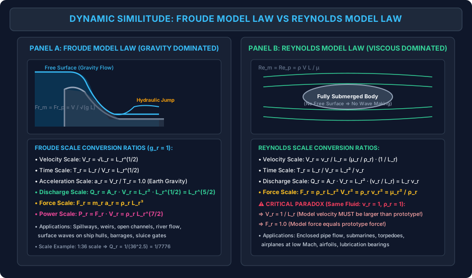
- Froude Model Law (): Governs all free-surface gravity flows (spillways, open channels, weirs, barrages, waves on ship hulls). Under standard gravity (), the scale ratios scale as:
- Reynolds Model Law (): Governs enclosed, fully submerged flows where viscous forces dominate (water transmission pipelines, submarines, low-speed airfoils, valves): (A critical physical paradox: If the same fluid is used in model and prototype, . A scale model must be tested at the prototype speed!)
Distorted Models in Civil River & Estuarine Hydraulics: When modeling vast natural rivers, reservoirs, and coastal estuaries (such as the Brahmaputra, Ganga, or Hooghly estuary), using an undistorted scale produces impractically shallow water depths (), where surface tension causes capillary meniscus clinging and flow artificially transitions into the laminar regime (). To maintain turbulent flow () and measurable water levels, civil engineers build Distorted Models possessing independent horizontal () and vertical () scale ratios, introducing a Vertical Exaggeration (typically to ). The corresponding Froude distorted scale ratios are:
3. Geometric, Kinematic & Dynamic Similitude
Complete hydraulic similitude between a model (subscript ) and prototype (subscript ) requires satisfying three hierarchical similarity conditions:
                  +---------------------------+
                  |    DYNAMIC SIMILITUDE     |
                  |    (Similarity of Forces) |
                  +-------------+-------------+
                                ^
                                | (Requires)
                  +-------------+-------------+
                  |   KINEMATIC SIMILITUDE    |
                  |   (Similarity of Motion)  |
                  +-------------+-------------+
                                ^
                                | (Requires)
                  +-------------+-------------+
                  |   GEOMETRIC SIMILITUDE    |
                  |   (Similarity of Shape)   |
                  +---------------------------+
3.1 Geometric Similarity (Similarity of Shape)
Geometric similarity implies that the model and prototype have identical physical shapes, with all corresponding linear dimensions scaled by a single, constant Scale Ratio ():
- Corresponding angles between surfaces are strictly equal: .
- Area Scale Ratio:
- Volume Scale Ratio:
3.2 Kinematic Similarity (Similarity of Motion)
Kinematic similarity implies that the streamline patterns in the model and prototype are geometrically similar, with the velocity and acceleration vectors at homologous (corresponding) points pointing in identical spatial directions with constant ratios:
- Velocity Scale Ratio:
- Time Scale Ratio:
- Acceleration Scale Ratio:
- Volumetric Discharge Scale Ratio:
3.3 Dynamic Similarity (Similarity of Forces)
Dynamic similarity requires that the ratios of all homologous active forces acting on fluid particles in model and prototype be identical:
where:
- : Inertia force,
- : Viscous shear force,
- : Gravitational weight force,
- : Pressure force,
- : Surface tension force,
- : Elastic compressibility force.
Because all fluid motions obey Newton's second law (), dynamic similarity is guaranteed if the ratio of Inertia Force to every other active force is identical between model and prototype.
4. The Five Primary Dimensionless Numbers & Force Ratios
Every primary dimensionless group in fluid mechanics represents the square root or direct ratio of Inertia Force () to another physical force mechanism:
4.1 Master Dimensionless Groups Table
| Dimensionless Number | Symbol | Mathematical Formulation | Force Ratio Definition | Governing Physical Regime / Civil Application |
|---|---|---|---|---|
| Reynolds Number | Enclosed pipe flow, laminar/turbulent transition, boundary layers, submarines, deep water tunnels | |||
| Froude Number | Free surface flows: Spillways, weirs, sluice gates, open channels, rivers, surface waves on ships | |||
| Euler Number | Flow with high localized pressure gradients, cavitation in siphons and turbines, pipe constrictions | |||
| Weber Number | Capillary phenomena, droplet atomization, thin sheet flow over aeration notches, micro-channels | |||
| Mach Number | High-velocity gas flows (), water hammer pressure transients in elastic penstocks |
5. Model Laws: Reynolds vs Froude Model Law Scale Derivations
In actual engineering testing, it is physically impossible to satisfy both Reynolds and Froude similarity simultaneously using water in both model and prototype (since requires while requires ). Engineers must identify the single predominant active force and design the model using the corresponding Model Law, while minimizing secondary forces through scale selection.
5.1 Froude Model Law ()
Applicable when gravity forces dominate and viscous/surface tension forces are negligible (free surface flows):
Under identical gravitational fields on Earth ():
- Velocity Scale Ratio ():
- Time Scale Ratio ():
- Acceleration Scale Ratio ():
- Discharge Scale Ratio ():
- Force Scale Ratio (): (If water is used in both model and prototype, ).
- Work / Energy Scale Ratio ():
- Power Scale Ratio ():
5.2 Reynolds Model Law ()
Applicable when viscous forces dominate and there is no free liquid surface:
- Velocity Scale Ratio ():
- Time Scale Ratio ():
- Discharge Scale Ratio ():
- Force Scale Ratio ():
The Reynolds Paradox (Identical Fluid: ): If the same fluid (e.g., water) is used in model and prototype:
Physical consequence: To test a scale submarine model in water, the model must be propelled at the prototype speed, and the drag force acting on the tiny model will equal the drag on the full-sized submarine! To avoid unmanageably high velocities, engineers test in pressurized variable-density wind tunnels or specialized heavy organic fluids (Freon/SF6) where kinematic viscosity .
6. Distorted Models in Civil Engineering: River, Estuary & Harbor Hydraulics
6.1 Undistorted vs Distorted Models Defined
- Undistorted Model: A model in which the geometric scale ratio is uniform in all directions: Used for structures with compact geometric aspect ratios: dam spillways, sluice gates, bridge piers, drop structures.
- Distorted Model: A model in which the horizontal scale ratio () and the vertical scale ratio () are deliberately chosen to be different: where .
6.2 Why Distortion is Essential for River and Harbor Models
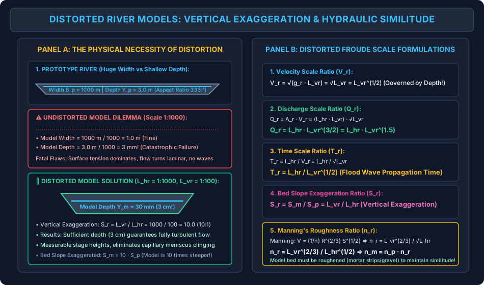
Consider a natural prototype river long, wide, and average depth. If built as an undistorted model at a practical horizontal scale of :
- Model length (manageable).
- Model width (manageable).
- Model water depth:
At a water depth of only :
- Surface Tension Dominance: Capillary meniscus clinging dominates; water forms isolated puddles and will not wet the bed properly.
- Laminar Flow Artifacts: The Reynolds number drops below , turning the flow laminar, whereas the real river is intensely turbulent ().
- Measurement Impossibility: Standard point gauges cannot measure water surface elevations with millimeter precision.
- Sediment Non-Transport: Silt and sand particles cannot move under laminar creeping boundary layers.
The Distorted Solution: Choose and .
- Model depth becomes .
- At depth, flow remains turbulent, surface tension is suppressed, and water levels can be measured with high precision!
6.3 Mathematical Scale Ratios for Distorted Froude Models
Because gravity drives open-channel river flow, Froude similitude is enforced using the vertical depth scale () as the characteristic length:
- Vertical Exaggeration (Distortion Ratio ): (The longitudinal bed slope of the model is exaggerated by ratio : ).
- Horizontal Area Scale Ratio ():
- Cross-Sectional Flow Area Scale Ratio ():
- Velocity Scale Ratio ():
- Discharge Scale Ratio ():
- Time Scale Ratio ():
- Manning's Roughness Scale Ratio (): Manning's equation states: . For wide channels, hydraulic radius . Bed slope ratio: . Substituting scale ratios: Equating with Froude velocity scale : (Because , . The laboratory model bed must be artificially roughened—using mortar ridges, wire mesh, or gravel studs—to achieve dynamic similitude!)
7. Scale Effects & Limitations of Hydraulic Scale Modeling
A Scale Effect is a systematic distortion or error between model predictions and prototype behavior resulting from the inability to satisfy multiple force ratios simultaneously.
Common Scale Effects in Civil Hydraulics:
- Viscous Scale Effects on Spillways: In an ogee spillway model sized by Froude law, the boundary layer along the chute is disproportionately thicker than in the prototype (). Consequently, the model slightly overpredicts skin friction loss and underpredicts crest discharge coefficients () by .
- Air Entrainment Scale Effects: Prototype high-velocity spillway chutes () entrain vast amounts of atmospheric air (white water bulking). Air entrainment is governed by the Weber Number () and turbulence intensity. Small-scale laboratory models underpredict air entrainment drastically because surface tension forces in the model prevent water surface tearing.
- Cavitation Scale Effects: Cavitation depends on absolute pressure head (). Because atmospheric pressure in the laboratory is unscaled (), scale models cannot reproduce cavitation unless placed inside specialized low-pressure vacuum flumes.
8. Visual Diagrams & Hydraulic Schematics
8.1 Froude vs Reynolds Model Laws Comparison
The multi-panel diagram below contrasts the physical regimes, dominant forces, and scale transformation ratios governing Froude free-surface flows against Reynolds enclosed viscous motions.
8.2 Distorted River Model Similitude & Scale Ratios
The schematic below illustrates the physical necessity of vertical exaggeration in wide, shallow alluvial rivers, presenting the complete geometric cross-sections and the governing Froude distorted scale formulas.
9. Step-by-Step Numerical Problems with Complete Calculations
Problem 1: Froude Model Law on Dam Spillway & Stilling Basin
Problem Statement: An ogee spillway and hydraulic jump stilling basin are modeled at an undistorted scale of ().
- The prototype spillway discharges a design flood of over a total crest width .
- The testing is conducted under Earth gravity () using fresh water ().
Calculate:
- Model discharge in and model crest width in ,
- If the water velocity entering the model stilling basin is measured as , calculate the prototype velocity in ,
- If the rate of hydraulic energy dissipation in the model jump is , calculate the prototype power dissipation in ,
- If a flood hydrograph of duration passes over the prototype dam, compute the corresponding model operating duration in hours and minutes.
Solution & Step-by-Step Calculation:
Step 1: Compute Froude Scale Ratios ()
- Velocity scale:
- Time scale:
- Discharge scale:
- Power scale:
Step 2: Model Discharge and Model Crest Width Model discharge:
Model crest width:
Step 3: Prototype Velocity in Stilling Basin
Step 4: Prototype Power Dissipation
Step 5: Model Flood Wave Duration
Problem 2: Reynolds Model Law — Submarine in Water Tunnel
Problem Statement: A prototype military submarine of length operates fully submerged in sea water () at cruising speed ().
- A scale model () is tested in a pressurized variable-density water tunnel using fresh water ().
- The drag force measured on the model in the tunnel is .
Calculate:
- Required water tunnel test velocity in ,
- Prototype drag force in ,
- Shaft propulsion power required by the prototype submarine in and .
Solution & Step-by-Step Calculation:
Step 1: Determine Required Model Velocity ()
Given: , , .
Step 2: Force Ratio and Prototype Drag Force Dynamic similarity requires equality of drag coefficients: .
Note that by Reynolds similarity: . Therefore:
Compute the force scale ratio:
Prototype drag force:
Step 3: Prototype Propulsion Power Required
Problem 3: Distorted River Model — Scales, Discharge & Roughness Adaptation
Problem Statement: A distorted movable-bed physical model is designed to investigate flood routing, bank erosion, and channel shoaling for a reach of an alluvial river.
- Horizontal scale: ().
- Vertical scale: ().
- Prototype river design flood discharge: .
- Prototype Manning's roughness coefficient: .
Determine:
- Vertical exaggeration of the model (),
- Velocity scale ratio ,
- Model discharge in ,
- Time scale ratio and the laboratory duration corresponding to a prototype flood hydrograph of duration ,
- Required Manning's roughness coefficient for the laboratory model bed.
Solution & Step-by-Step Calculation:
Step 1: Vertical Exaggeration ()
Step 2: Velocity Scale Ratio () Based on Froude similitude governed by vertical depth :
Step 3: Discharge Scale Ratio and Model Discharge
Model discharge:
Step 4: Time Scale Ratio and Model Duration
Model hydrograph duration:
(A 2-day prototype flood wave passes through the model in under 29 minutes!)
Step 5: Model Manning's Roughness Coefficient ()
Required model bed roughness:
(Because , smooth cement plaster () cannot be used; the model bed must be artificially roughened with wire mesh, exposed gravel, or cross-ribs to maintain dynamic flow similitude).
10. High-Yield Exam Pitfalls, Traps & Shortcuts
-
Froude Discharge Scaling ( vs ):
- Trap: Calculating model discharge as .
- Truth: Volume scales as , but volumetric discharge is volume per unit time (), so .
-
The "Reynolds Scale Model Force Equals Prototype Force" Paradox:
- Trap: Thinking a tiny submarine model experiences a negligible fraction of prototype drag.
- Truth: If the same fluid is used in model and prototype (), . The drag on the small model is identical to the drag on the massive prototype ().
-
Distorted Model Discharge Scale ():
- Trap: Using or in a distorted model.
- Truth: Flow area is . Velocity is . Therefore, .
-
Time Scale in Distorted Models ():
- Time is horizontal distance divided by velocity: . Never use !
-
Dominant Force Recognition for Model Law Selection:
- Free surface / Spillway / Weirs / Open Channel Froude Law ().
- Enclosed pipe / Viscous drag / Submerged submarine Reynolds Law ().
- High-speed gas / Shock waves / Water hammer Mach Law ().
- Capillary / Thin liquid film / Atomization Weber Law ().
- Cavitation in hydraulic machines Euler Law ().
11. Multi-Exam Question Bank (GATE, ESE, SSC JE, State AE, RRB JE)
Question 1 (GATE CE — Multiple Choice Question)
A scale model of a spillway is to be tested in a laboratory. The prototype discharge is . If the Froude model law governs the flow, the discharge to be maintained in the model is:
- A)
- B)
- C)
- D)
Detailed Solution: Froude discharge scale ratio:
Model discharge:
Matching option B. Correct Answer: B
Question 2 (UPSC ESE Paper-II)
In a distorted river model, the horizontal scale is and the vertical scale is . If a flood discharge of passes through the prototype river, the corresponding discharge in the model should be:
- A)
- B)
- C)
- D)
Detailed Solution: , .
Model discharge:
Correct Answer: B
Question 3 (SSC JE)
Kinematic similarity between model and prototype exists when:
- A) Linear dimensions are in a constant ratio
- B) The streamline patterns are geometrically similar and velocity ratios at corresponding points are equal
- C) Ratios of all corresponding forces are equal
- D) Masses and densities are identical
Detailed Solution:
- Geometric similarity: Similarity of shape/lengths.
- Kinematic similarity: Similarity of motion (streamlines, velocity vectors, acceleration).
- Dynamic similarity: Similarity of forces. Correct Answer: B
Question 4 (State PSC AE)
A ship model of scale is tested in a towing tank according to Froude's law. If the wave resistance on the model is measured as , the wave resistance on the prototype ship will be:
- A)
- B)
- C)
- D)
Detailed Solution: Under Froude law with same water density ():
Prototype force:
Correct Answer: C
Question 5 (RRB JE)
The dimensionless number that governs the phenomenon of cavitation in hydraulic machinery is:
- A) Mach number
- B) Euler number
- C) Weber number
- D) Froude number
Detailed Solution: Cavitation occurs when local pressure drops to vapor pressure, driven by intense pressure gradients. The Euler number () or cavitation parameter represents the ratio of inertia force to pressure force and governs cavitation. Correct Answer: B
12. Comprehensive Summary, Formula Cheatsheet & Academic References
Master Formula Cheatsheet
Academic References & Standard Source Texts
- White, F. M. (2016). Fluid Mechanics (8th ed.). McGraw-Hill Education. Chapter 5: Dimensional Analysis and Similarity (Sections 5.4 & 5.5: Modeling and Similitude).
- Modi, P. N., & Seth, S. M. (2018). Hydraulics and Fluid Mechanics Including Hydraulics Machines (22nd ed.). Standard Book House, New Delhi. Chapter 13: Model Analysis.
- Streeter, V. L., Wylie, E. B., & Bedford, K. W. (1998). Fluid Mechanics (9th ed.). WCB/McGraw-Hill. Chapter 5: Dynamic Similitude and Model Studies.
- Rajput, R. K. (2020). A Textbook of Fluid Mechanics and Hydraulic Machines (7th ed.). S. Chand & Company Ltd. Chapter 12: Model Analysis.
- Central Water and Power Research Station (CWPRS): Technical Manual on River and Estuarine Physical Hydraulic Modeling. Pune, Ministry of Jal Shakti.