Minor Losses, Compound Pipes, Parallel Pipes & Pipe Networks (Hardy Cross Method)
In this chapter (4 topics)
On this page
- 1. Module Overview & Pedagogical Scope
- 2. Official Examination Syllabus Mapping
- 3. Fundamental Physical Principles & Governing Assumptions
- 4. Mathematical Derivations & Rigorous Proofs
- Sub-derivation A: Sudden Expansion (Borda-Carnot Theorem)
- Sub-derivation B: Sudden Contraction & Vena Contracta Dissipation
- Sub-derivation C: Minor Loss Coefficients Catalog
- Sub-derivation D: Compound Pipes in Series & Dupuit's Equivalent Pipe Formulation
- Sub-derivation E: Parallel Pipes & Discharge Division
- Sub-derivation F: Pipe Networks & The Hardy Cross Method
- 5. Technical Diagrams & Interactive Architectural Schematics
- Figure 1: Minor Losses at Expansions, Contractions & Standard Fittings
- Figure 2: Compound Pipe Systems & Hardy Cross Loop Balancing
- 6. Comparative Engineering Analysis & Parameter Regimes
- 7. Worked Numerical Examples (Pre-Calculated & Verified)
- Problem 1: Compound Pipe in Series & Dupuit's Equivalent Pipe
- Problem 2: Parallel Pipes & Flow Distribution
- Problem 3: Hardy Cross Network Loop Balancing
- 8. High-Yield Examination Traps & Ambiguities
- 9. Real-World Engineering Applications & Case Studies
- 10. Cross-Disciplinary & Downstream Dependencies
- 11. Summary Formula Cheat Sheet & Memory Anchors
- 12. Comprehensive References & Standard Codes
1. Module Overview & Pedagogical Scope
In civil and environmental hydraulic engineering, pipelines rarely consist of single, straight, uninterrupted uniform conduits. Municipal water distribution grids, sewage pumping mains, industrial plant plumbing, and hydroelectric penstocks incorporate numerous geometric transitions, pipe fittings, valves, bends, expansions, contractions, bifurcations, and interconnected closed loops.
Head losses in pipe systems are classified into two fundamental thermodynamic categories:
- Major Head Losses (): Frictional resistance generated continuously along the wetted perimeter over the conduit length, governed by the Darcy-Weisbach formulation.
- Minor Head Losses (): Localized dissipation of mechanical energy caused by intense boundary layer separation, turbulent eddy generation, and momentum reassessment at geometric discontinuities (pipe entrances, sudden expansions, sudden contractions, bends, tees, and control valves).
This module delivers an exhaustive analytical, mathematical, and algorithmic treatment of:
- Exact hydrodynamic momentum proofs for sudden expansion (Borda-Carnot theorem) and sudden contraction (vena contracta dissipation).
- Catalog of standardized empirical component loss coefficients ().
- Flow through compound pipelines in series and Dupuit's equivalent pipe formulation.
- Splitting of discharge across parallel conduit branches and branched three-reservoir networks.
- Iterative loop relaxation algorithm for complex closed-loop water distribution networks via the Hardy Cross Method using both Darcy-Weisbach and Hazen-Williams resistance formulations.
2. Official Examination Syllabus Mapping
Website note: this mapping is from the author’s notes. It has not been checked against the official notification for each examination; confirm the current syllabus with the examining body.
| Examination Body | Syllabus Clause / Core Topic Reference | Focus Regimes & Weightage |
|---|---|---|
| GATE CE (IITs / IISc) | Fluid Mechanics: Losses in pipe flow (major and minor losses); pipe network analysis; equivalent pipe; pipes in series and parallel; Hardy Cross method. | High Weightage (1 to 2 questions every year; equivalent length calculations, parallel pipe discharge division, loop flow correction ). |
| UPSC ESE (Prelims & Mains) | Paper-II Fluid Mechanics: Minor losses, sudden enlargement and contraction, pipes in series and parallel, branched pipes, Hardy Cross loop balancing method. | Core Conventional & Objective Subject (15–20 marks in Mains; 2–4 MCQs in Prelims). |
| SSC JE & State AE / JE | Loss of head due to sudden enlargement, contraction, obstruction; pipes in series and parallel; equivalent pipe length; Dupuit’s equation. | Extremely High Frequency (Direct formula questions on Borda-Carnot, for entrance, Dupuit's ). |
| RRB JE (CBT-2) | Fluid flow through pipes, minor losses, equivalent pipe concept. | Standard numericals and concept-based MCQs. |
3. Fundamental Physical Principles & Governing Assumptions
- Energy Conservation (Extended Bernoulli Theorem): The total piezometric plus kinetic energy head between any two sections 1 and 2 is conserved after accounting for cumulative major and minor losses:
- Proportionality to Kinetic Head: Minor head losses are mathematically parameterized as fractions of the local kinetic velocity head: where is the dimensionless minor loss coefficient. For transitions between conduits of different diameters, is strictly keyed to a specifically referenced velocity (typically the downstream or higher-velocity conduit).
- Kirchhoff's Hydraulic Analogues for Networks:
- Junction Law (Continuity): The algebraic sum of discharges entering and leaving any conduit junction node is identically zero:
- Loop Law (Uniqueness of Head): The algebraic sum of piezometric head losses around any closed hydraulic loop must vanish identically:
4. Mathematical Derivations & Rigorous Proofs
Sub-derivation A: Sudden Expansion (Borda-Carnot Theorem)
Consider a steady, incompressible flow expanding abruptly from an upstream pipe of area and velocity to a downstream pipe of area and velocity ().
1. Flow Field & Control Volume Definition
As the fluid emerges from the smaller conduit, it forms an expanding submerged jet. Because of the abrupt boundary geometry, the fluid cannot follow the sharp corners, resulting in severe boundary layer separation and establishing recirculating dead-water eddy zones in the annular clearance between and .
Isolate a control volume bounded by Section 1-1 immediately at the expansion plane and Section 2-2 sufficiently downstream where the flow has reattached and uniform parallel streamlines have re-established.
2. Experimental Boundary Condition
Experiments (corroborated by potential flow theory) show that the pressure acting on the annular vertical step area is virtually uniform and equal to the incoming jet pressure :
3. Linear Momentum Balance
Applying the integral linear momentum equation along the longitudinal flow axis:
Simplifying the left-hand side:
Therefore:
Substitute :
Dividing by and dividing by specific weight :
4. Extended Bernoulli Energy Equation
Applying the energy equation across Sections 1-1 and 2-2 for a horizontal conduit ():
Substituting the pressure head difference from the momentum balance:
This is the celebrated Borda-Carnot Formula for head loss due to sudden enlargement.
Expressing in terms of upstream velocity via continuity ():
Special Limiting Case (Pipe Exit into Reservoir):
When a pipe discharges into a large reservoir, .The entire kinetic energy head is completely dissipated as heat through turbulent eddy decay!
Sub-derivation B: Sudden Contraction & Vena Contracta Dissipation
When fluid flows abruptly from a large pipe of area to a smaller pipe of area (), the converging streamlines cannot negotiate the sharp corner, causing separation and converging into a contracted jet throat called the vena contracta at Section inside the smaller conduit.
- Area at vena contracta: , where is the coefficient of contraction.
- From Section 1-1 to , the flow accelerates under a favorable pressure gradient; energy loss is negligible.
- From Section to downstream uniform Section 2-2, the jet expands abruptly under an adverse pressure gradient, producing severe turbulent eddy dissipation identical to a sudden enlargement!
Applying the Borda-Carnot formula between Section and Section 2-2:
By continuity: . Substituting :
For standard commercial pipes where :
If (sharp-edged entrance from a reservoir), :
Sub-derivation C: Minor Loss Coefficients Catalog
| Fitting / Discontinuity Type | Physical Mechanism | Dimensionless Coefficient () |
|---|---|---|
| Bell-Mouthed / Rounded Entrance | Streamlines smoothly guide without separation | |
| Sharp-Edged Flush Entrance | Separation and vena contracta () | |
| Re-entrant (Borda) Entrance | Inward projecting pipe creates severe contraction () | |
| Submerged Reservoir Pipe Exit | Total kinetic energy dissipated in receiving basin | |
| Standard Threaded Elbow | Secondary twin-vortex swirling and separation | |
| Long-Radius Flanged Bend | Curvature minimizes secondary vortex generation | |
| Standard Elbow | Moderate turning separation | |
| Tee Junction (Flow Along Run) | Minimal diversion turbulence | |
| Tee Junction (Flow Diverted to Branch) | Extreme perpendicular deceleration and swirl | |
| Gate Valve (Fully Open) | Unobstructed full-bore waterway | |
| Gate Valve ( Open) | Partial throttling | |
| Gate Valve ( Open) | Severe throttling | |
| Gate Valve ( Open) | Extreme throttling | |
| Globe Valve (Fully Open) | S-shaped tortuous internal fluid passage | |
| Swing Check Valve (Fully Open) | Disc drag in fluid stream |
Sub-derivation D: Compound Pipes in Series & Dupuit's Equivalent Pipe Formulation
When a pipeline consists of multiple pipes of different lengths (), diameters (), and friction factors () connected end-to-end in series:
- Continuity Law: The volumetric flow rate through every segment is identical:
- Energy Conservation: Total head loss is the cumulative sum of major and minor losses:
Expressing velocity in terms of discharge: . Substituting into the Darcy major friction loss equation:
Dupuit's Equivalent Pipe:
An equivalent pipe is defined as an imaginary pipe of uniform diameter , uniform length , and friction factor that conveys the exact same discharge under the exact same total head loss .
Equating total major friction loss:
Canceling the common factor :
If all pipes are of the same material (), this reduces to Dupuit's Classical Equation:
Sub-derivation E: Parallel Pipes & Discharge Division
When a main pipeline splits at upstream junction into parallel branches that reunite at downstream junction :
- Continuity Law: Total inflow equals the sum of branch discharges:
- Head Loss Identity: The piezometric head at junction is and at junction is . Therefore, the head loss across every single parallel branch is identical:
Expressing head loss in pipe resistance form ( where ):
Critical Examination Rule: In parallel pipes, flow divides such that the branch with larger diameter carries a vastly disproportionate share of the flow, scaling as !
Sub-derivation F: Pipe Networks & The Hardy Cross Method
Water distribution networks in cities consist of complex loops. In 1936, Professor Hardy Cross developed a systematic relaxation method based on successive corrections:
1. Governing Equations:
- Node Continuity: At every junction: .
- Loop Energy Balance: Around every closed loop: , where:
- For Darcy-Weisbach: , (with ).
- For Hazen-Williams: , (with ).
2. Derivation of the Loop Flow Correction ():
Assume an initial trial flow distribution in every pipe that strictly satisfies junction continuity (). Due to initial estimation errors, the loop head loss will not balance:
Let be the true, unknown constant flow correction applied uniformly around the closed loop (defined positive in the clockwise sense). The true discharge in each pipe is . Enforcing loop energy equilibrium:
Expanding using Taylor's binomial series:
Since , the second-order term is negligibly small and discarded:
For the general head loss law :
Sign Convention:
- Flows circulating clockwise around the loop produce positive head loss ().
- Flows circulating counter-clockwise produce negative head loss ().
- The denominator is strictly positive (absolute sum).
- For a pipe common to two adjacent loops, it receives corrections from both loops:
5. Technical Diagrams & Interactive Architectural Schematics
Figure 1: Minor Losses at Expansions, Contractions & Standard Fittings
The diagram below presents the Borda-Carnot momentum balance on a sudden expansion, the vena contracta formation during sudden contraction, and the catalog of standard component loss coefficients.
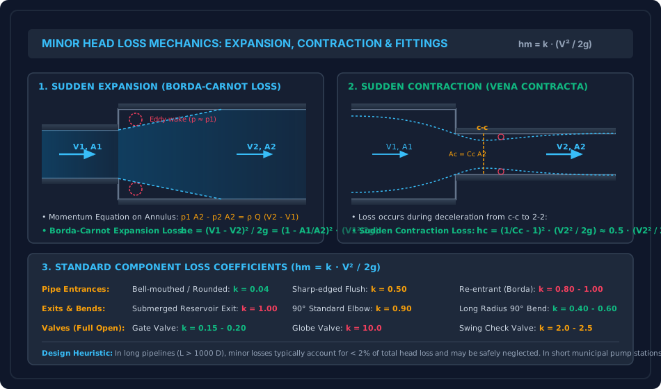
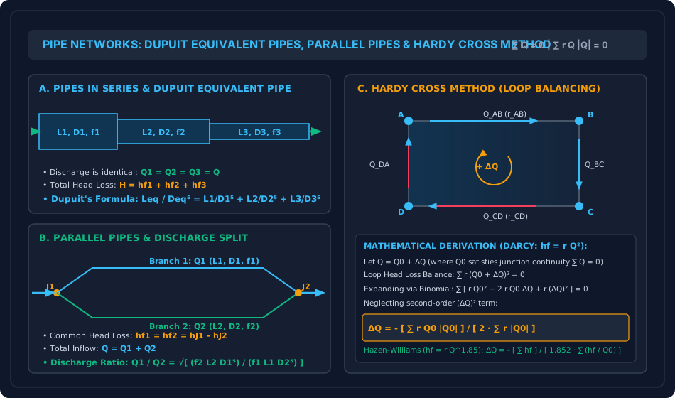
Figure 2: Compound Pipe Systems & Hardy Cross Loop Balancing
The diagram below contrasts compound pipes in series (Dupuit equivalent formulation), parallel pipes (equal head loss across branches), and closed-loop Hardy Cross network relaxation.
6. Comparative Engineering Analysis & Parameter Regimes
| Network Architecture | Flow Continuity Law | Energy / Head Loss Law | Governing Equations | Civil Engineering Application |
|---|---|---|---|---|
| Compound Pipes in Series | (Constant) | (Dupuit) | Long-distance transmission mains, rising mains from pump house. | |
| Parallel Pipes | (Flow divides) | (Identical) | Pipeline looping to augment carrying capacity, river crossings. | |
| Three-Reservoir Branched | Piezometric head at junction dictates flow direction | Regional water distribution from multiple elevated service reservoirs. | ||
| Closed-Loop Grid Network | at all nodes | around all loops | Municipal urban distribution grids (looped system prevents stagnation). |
7. Worked Numerical Examples (Pre-Calculated & Verified)
Problem 1: Compound Pipe in Series & Dupuit's Equivalent Pipe
Statement:
Two reservoirs have a water surface elevation difference of . They are connected by a compound pipeline of total length consisting of three commercial pipes in series:
- Pipe 1: (), Darcy
- Pipe 2: (), Darcy
- Pipe 3: (), Darcy
Minor losses include: sharp entrance (), sudden contraction from Pipe 1 to 2 (), sudden contraction from Pipe 2 to 3 (), and submerged exit into reservoir 2 ().
- Determine the flow rate through the pipeline considering both major and minor losses.
- Determine the flow rate if all minor losses are neglected, and compute the percentage error.
- Compute the Dupuit equivalent length of a uniform pipe having diameter and .
Solution:
Step 1: Pipeline Resistance Factors Expressing major head losses as where :
Total major friction resistance:
Step 2: Minor Losses Formulation
- Entrance loss:
- Contraction 1 to 2:
- Contraction 2 to 3:
- Exit loss: Total minor resistance:
Total system resistance:
Step 3: Discharge Determination
- Considering all losses:
- Neglecting minor losses:
- Percentage discrepancy:
(Confirms that for pipelines longer than , minor losses are well under ).
Step 4: Dupuit's Equivalent Length ()
Problem 2: Parallel Pipes & Flow Distribution
Statement:
A municipal distribution trunk divides at junction into two parallel branches that reunite at downstream junction :
- Branch 1: (),
- Branch 2: (),
The total discharge entering junction is ().
- Calculate the pipe resistance coefficients and .
- Determine the discharge carried by Branch 1 () and Branch 2 ().
- Compute the common friction head loss between junctions and .
Solution:
Step 1: Resistance Coefficients ()
Step 2: Flow Splitting Ratio Since head loss is identical ():
By continuity: :
Step 3: Head Loss Verification
(Exact match confirmed to 4 decimal places).
Problem 3: Hardy Cross Network Loop Balancing
Statement:
A closed square pipe loop has four pipe lines with known resistance constants ( in ) and initially assumed flow rates :
- Pipe : , assumed (clockwise)
- Pipe : , assumed (clockwise)
- Pipe : , assumed (counter-clockwise)
- Pipe : , assumed (counter-clockwise)
- Check whether loop energy is balanced under the initial flow assumptions.
- Calculate the loop flow correction after the first Hardy Cross iteration.
- Compute the corrected flow rates in all four pipes.
Solution:
Step 1: Head Loss & Derivative Evaluation (Hardy Cross Table)
| Pipe | Resistance | Assumed () | Sense | Head Loss () | Derivative |
|---|---|---|---|---|---|
| Clockwise () | |||||
| Clockwise () | |||||
| Counter-CW () | |||||
| Counter-CW () | |||||
| Sum () | — | — | — |
Step 2: Loop Flow Correction Calculation
(Since was negative, counter-clockwise flow was dominant; is positive, adding clockwise flow to balance the loop).
Step 3: Corrected Flow Rates after Iteration 1
- Pipe :
- Pipe :
- Pipe :
- Pipe :
8. High-Yield Examination Traps & Ambiguities
| S.No. | Examination Trap / Ambiguity | Correct Technical Reality | Examination Body |
|---|---|---|---|
| 1 | Borda-Carnot Velocity Reference: Taking vs . | The loss is proportional to the squared difference of velocities , NOT . | GATE CE, SSC JE |
| 2 | Contraction Velocity Reference: Using upstream velocity for sudden contraction loss. | Contraction loss is strictly keyed to downstream velocity in the smaller pipe, where vena contracta deceleration occurs. | GATE CE, UPSC ESE |
| 3 | Hardy Cross Denominator Sign: Taking algebraic signs in the denominator . | The denominator of Hardy Cross is strictly positive: . Applying negative signs in the denominator causes catastrophic divergence. | GATE CE, ESE Mains |
| 4 | Common Pipe Correction in Two Loops: Forgetting that common pipes carry corrections from both loops. | For a pipe shared between Loop I and Loop II: (assuming both loops define clockwise as positive). | UPSC ESE, GATE CE |
| 5 | Dupuit's Exponent: Using instead of . | Since discharge , head loss . Therefore, Dupuit's equivalent length strictly scales as (not ). | SSC JE, State AE |
9. Real-World Engineering Applications & Case Studies
- Urban Water Supply Grid Reliability:
Municipal water distribution systems are laid out as looped grid networks analyzed via Hardy Cross algorithms. If a water main breaks or is isolated for maintenance, looped hydraulics ensure that downstream consumer demand nodes continue receiving supply from alternate directions without interruption. - Hydraulic Surge Suppression & Valve Closure Stations:
Water treatment plants and raw water transmission mains install check valves and air release valves at high points. Calculating minor head losses across multi-turn gate valves and motorized butterfly valves dictates pump selection and motor horsepower. - Pumping Main Looping for Capacity Augmentation:
When a rising water main reaches capacity due to urban growth, civil authorities construct a parallel "loop" along a fraction of the pipeline length. As proven in Problem 2, adding a parallel branch drastically reduces resistance and boosts discharge without requiring full pipeline replacement.
10. Cross-Disciplinary & Downstream Dependencies
[Fluid Mechanics: Ch 06 Topic 03 Minor Losses & Networks]
        │
        ├──► [Subject 09: Environmental Engineering]
        │         ├─► Design of Municipal Water Supply Distribution Systems
        │         ├─► Hardy Cross Loop Simulation in EPANET
        │         └─► Booster Chlorination & Pumping Station Head Calculations
        │
        ├──► [Subject 04: Water Resources & Hydrology]
        │         └─► Hydropower Penstock Manifolds & Bifurcations
        │
        └──► [Fluid Mechanics: Ch 06 Topic 04]
                  └─► Water Hammer Pressure Surges Triggered by Valve Closure
11. Summary Formula Cheat Sheet & Memory Anchors
- Sudden Expansion (Borda-Carnot):
- Sudden Contraction:
- Pipe Entrance & Exit:
- Dupuit's Equivalent Pipe:
- Parallel Pipes:
- Hardy Cross Method:
12. Comprehensive References & Standard Codes
- Cross, Hardy (1936). Analysis of Flow in Networks of Conduits or Conductors, University of Illinois Engineering Experiment Station Bulletin No. 286.
- CPHEEO Manual on Water Supply and Treatment (Ministry of Housing and Urban Affairs, Government of India).
- White, F. M. (2016). Fluid Mechanics, 8th Edition, McGraw-Hill Education.
- Streeter, V. L., & Wylie, E. B. (1998). Fluid Mechanics, 9th Edition, McGraw-Hill.
- IS 5330:1984 (Criteria for Design of Anchor Blocks for Penstocks Along Slopes).