Velocity Potential Function, Stream Function, Laplace Equation & Flow Nets
In this chapter (5 topics)
On this page
- 1. Topic Metadata Table
- 2. Executive Summary
- 3. Velocity Potential Function (φ) & Irrotational Potential Flow
- 3.1 Mathematical Definition & Sign Convention
- 3.2 Necessary and Sufficient Condition for Existence: Irrotationality
- 3.3 Governing Equation: The Laplace Equation
- 4. Stream Function (ψ) & Incompressible 2D Continuity
- 4.1 Mathematical Definition
- 4.2 Proof of Automatic Continuity Satisfaction
- 4.3 Physical Significance: Volumetric Discharge Between Streamlines
- 4.4 Irrotationality & The Laplace Equation for ψ
- 5. Cauchy-Riemann Relations, Complex Potential & Orthogonality
- 5.1 Cauchy-Riemann Equations
- 5.2 Complex Velocity Potential W(z)
- 5.3 Mathematical Proof of Mutual Orthogonality
- 6. Flow Net Theory & Properties
- 6.1 Essential Properties of an Ideal Flow Net
- 7. Civil Engineering Applications: Seepage & Piping Analysis
- 7.1 Seepage Discharge Formulation
- 7.2 Exit Hydraulic Gradient & Piping (Quicksand) Failure
- 8. Visual Diagrams & Architectural Schematics
- 8.1 Potential Flow Theory: φ & ψ Orthogonality & Laplace Grid
- 8.2 Flow Net Seepage Under Concrete Weir / Dam & Piping Stability
- 9. Step-by-Step Numerical Problems with Complete Calculations
- Problem 1: Velocity Potential, Conjugate Stream Function & Flow Rate
- Problem 2: Cubic Stream Function, Complex Potential & Flow Classification
- Problem 3: Seepage Flow Net Under a Concrete Dam with Sheet Pile Cutoff
- 10. High-Yield Exam Pitfalls, Traps & Shortcuts
- 11. Multi-Exam Question Bank (GATE, ESE, SSC JE, State AE, RRB JE)
- Question 1 (GATE CE — Analytical)
- Question 2 (UPSC ESE Paper-II — Descriptive / Analytical)
- Question 3 (SSC JE — Direct Conceptual)
- Question 4 (State PSC AE — Numerical)
- Question 5 (RRB JE — Direct Knowledge)
- 12. Comprehensive Summary, Formula Cheatsheet & Academic References
- 12.1 Formula Cheatsheet
- 12.2 Academic & Standard References
1. Topic Metadata Table
| Field | Detail |
|---|---|
| Subject | Fluid Mechanics & Hydraulic Machinery (Subject 07) |
| Chapter | Chapter 03: Fluid Kinematics |
| Topic Code | FM-03-05 |
| Topic Title | Velocity Potential Function (), Stream Function (), Cauchy-Riemann Equations, Laplace Equation, Orthogonality & Flow Nets |
| Prerequisites | FM-03-01 (Flow Classification), FM-03-02 (Continuity Equation), FM-03-04 (Vorticity, Rotation & Circulation), Complex Analysis (Analytic Functions) |
| Target Examinations | GATE CE, UPSC ESE (Paper-II), SSC JE, State PSC AE/JE, RRB JE |
| Knowledge Level | Fundamental Potential Theory to Advanced Geotechnical/Hydraulic Seepage Analysis |
| IS / IRC / Standard Codes | IS 4880 (Code of practice for design of tunnels, hydraulic aspects), IS 8414 (Guidelines for design of under-seepage control measures for earth and rockfill dams), IS 7784 |
| Key Formulae | , , , , , , , |
2. Executive Summary
Potential flow theory forms the mathematical core of classical fluid kinematics, providing exact analytical solutions for two-dimensional and three-dimensional ideal fluid motions, as well as groundwater seepage through porous geotechnical media. Two scalar potential functions govern this framework:
- Velocity Potential Function (): Defined such that its negative gradient yields the velocity vector:
(The negative sign is the standard civil engineering convention, ensuring that flow naturally proceeds from higher potential to lower potential).
- Existence Condition: The velocity potential function exists if and only if the flow is irrotational ().
- When combined with the incompressible continuity equation (), satisfies the Laplace Equation:
- A function satisfying the Laplace equation is called a Harmonic Function.
- Stream Function (): Formulated specifically for two-dimensional continuous flows such that it identically satisfies the 2D continuity equation:
- Existence Condition: The stream function exists if and only if continuity is satisfied (). It exists for both rotational and irrotational 2D flows.
- If the flow is additionally irrotational (), also satisfies the Laplace Equation:
When both and satisfy the Laplace equation, they form a pair of conjugate harmonic functions linked by the Cauchy-Riemann Equations:
and define an analytic complex potential function , where .
A cornerstone physical property is that Equipotential Lines () and Streamlines () intersect each other at strict right angles ( orthogonality) everywhere in the flow field, except at stagnation points where velocity is zero. Graphically, this orthogonal intersection forms a Flow Net composed of curvilinear squares. In civil hydraulic and geotechnical engineering, flow nets provide precise solutions for seepage discharge under concrete gravity dams and weirs (), hydrostatic uplift pressure distributions, exit hydraulic gradients (), and safety factors against catastrophic piping or quicksand failure ().
3. Velocity Potential Function () & Irrotational Potential Flow
3.1 Mathematical Definition & Sign Convention
The Velocity Potential Function is a scalar spatial function whose partial derivative with respect to any displacement coordinate gives the fluid velocity component along that coordinate direction.
In standard civil engineering and hydraulic conventions:
In compact vector calculus notation:
Sign Convention Note: In some classical mathematics texts, is used. In engineering hydraulics and hydrogeology, the negative sign is universally adopted because fluid moves spontaneously from regions of high potential (energy head) toward regions of lower potential, matching Darcy's law and Fourier's law.
3.2 Necessary and Sufficient Condition for Existence: Irrotationality
Consider the curl of the velocity vector:
From vector calculus, the curl of any gradient field is identically zero:
Therefore:
If a flow field has non-zero vorticity (, such as in a boundary layer, turbulent wake, or forced vortex), no velocity potential function can exist.
3.3 Governing Equation: The Laplace Equation
Substitute the velocity components into the 3D incompressible continuity equation:
Key Properties of :
- It is a linear partial differential equation. By the Principle of Superposition, any linear combination of valid potential flows is also a valid potential flow (e.g., Uniform flow + Source/Sink = Flow past a Rankine half-body; Uniform flow + Doublet = Flow past a circular cylinder).
- Any function satisfying represents a physically possible steady or unsteady incompressible irrotational flow field.
- It applies to both 2D and 3D flows.
4. Stream Function () & Incompressible 2D Continuity
4.1 Mathematical Definition
The Stream Function is a scalar function defined for two-dimensional continuous flows such that lines along which represent streamlines.
In standard Cartesian coordinates:
4.2 Proof of Automatic Continuity Satisfaction
Substitute and into the 2D incompressible continuity equation:
By Schwarz's theorem for continuous mixed partial derivatives, . Thus:
Conclusion: Any continuous, differentiable stream function automatically satisfies the 2D incompressible continuity equation, whether the flow is rotational or irrotational!
4.3 Physical Significance: Volumetric Discharge Between Streamlines
Consider two streamlines and . Let be an arbitrary line segment connecting them. The volumetric discharge crossing an elementary segment of length with normal components and is:
Substitute and :
Integrating between point on streamline and point on streamline :
Fundamental Principle: The volumetric discharge per unit width () flowing between any two streamlines is simply the algebraic difference of their stream function values, regardless of the shape or path connecting them.
4.4 Irrotationality & The Laplace Equation for
While exists for any 2D flow satisfying continuity, it satisfies the Laplace equation only when the flow is irrotational. The -component of vorticity is:
Substitute and :
For irrotational flow, :
5. Cauchy-Riemann Relations, Complex Potential & Orthogonality
5.1 Cauchy-Riemann Equations
When a 2D flow field is both incompressible () and irrotational (), both and exist simultaneously. Equating the velocity expressions:
These are the classical Cauchy-Riemann Differential Equations of complex analysis. (Note: If the convention is used, they take the standard textbook form and ).
5.2 Complex Velocity Potential
Because and satisfy the Cauchy-Riemann equations, they can be unified into a single holomorphic (analytic) function of the complex variable :
where:
- is the velocity potential.
- is the stream function.
Differentiating with respect to yields the Complex Velocity:
5.3 Mathematical Proof of Mutual Orthogonality
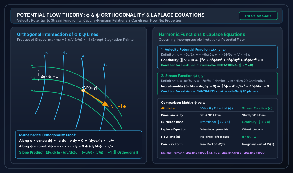
An equipotential line is defined by . Taking its total differential:
The slope of the equipotential line () is:
A streamline is defined by . Taking its total differential:
The slope of the streamline () is:
Multiplying the two slopes:
Conclusion: Because the product of their slopes is , Equipotential lines and Streamlines intersect at right angles ( orthogonality) everywhere in the flow field.
Stagnation Point Exception:
At a stagnation point, the fluid velocity is zero: and . The slopes and become mathematically indeterminate. The Cauchy-Riemann mapping ceases to be conformal at stagnation points, and streamlines and equipotentials may meet at angles other than (for instance, branching at where is the order of the stagnation singularity).
6. Flow Net Theory & Properties
A Flow Net is a graphical grid formed by the orthogonal intersection of a family of streamlines and a family of equipotential lines.
       ψ_4 ───────────────────────────────────────── (Streamline)
            │         │         │         │
            │  Cell   │  Cell   │  Cell   │  b
            │         │         │         │
       ψ_3 ─────────────────────────────────────────
            │    a    │         │         │
            │◄───────►│         │         │
            │         │         │         │
       ψ_2 ─────────────────────────────────────────
           ϕ_1       ϕ_2       ϕ_3       ϕ_4
                 (Equipotential Lines)
6.1 Essential Properties of an Ideal Flow Net
- Curvilinear Squares: The lines are drawn such that the spacing between adjacent streamlines () and adjacent equipotential lines () is approximately equal: A true circle can be inscribed tangent to all four curved boundary segments of every interior cell.
- Equal Potential Drop (): The total head loss is subdivided into equal intervals:
- Equal Discharge per Channel (): The total flow rate is divided equally among flow channels:
- Boundary Conditions:
- Solid Impermeable Boundaries: (e.g., dam concrete base, sheet pile wall, impermeable bedrock floor) are streamlines (). Flow cannot penetrate across them; equipotential lines must meet them at right angles ().
- Pervious Ground Boundaries: (e.g., upstream reservoir bed, downstream tailwater bed) are equipotential lines (). Streamlines must enter or exit them perpendicularly.
- Phreatic (Free Surface) Line in Earth Dams: The upper boundary of seepage is a streamline () on which pressure is atmospheric ().
7. Civil Engineering Applications: Seepage & Piping Analysis
7.1 Seepage Discharge Formulation
Consider one curvilinear cell of length along the flow direction and width perpendicular to flow. By Darcy's Law:
where is the coefficient of soil permeability and unit width () into the plane is considered. Rearranging:
For curvilinear squares, the aspect ratio is unity: .
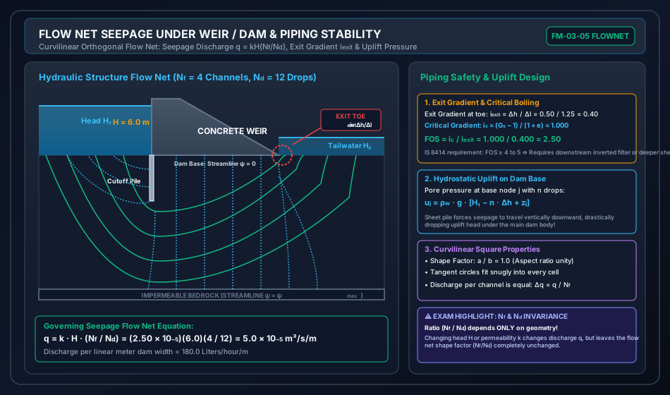
The total seepage discharge across all flow channels is:
The dimensionless ratio is known as the Shape Factor of the flow net. It depends solely on the boundary geometry of the structure and is completely independent of the hydraulic head or soil permeability .
7.2 Exit Hydraulic Gradient & Piping (Quicksand) Failure
As water seeps upward toward the downstream bed level, it exerts an upward drag (seepage force) on the soil grains. The Exit Hydraulic Gradient () occurs across the final equipotential field element of length adjacent to the downstream toe:
Critical Hydraulic Gradient ():
When the upward seepage force exactly balances the submerged (effective) unit weight of the soil grains, the effective stress drops to zero:
For typical quartz sands (), .
Factor of Safety Against Piping ():
According to IS 8414 and IS 4880, to prevent boil formation, progressive piping, and structural collapse:
- Silt foundations: to ( to ).
- Fine sand: to ( to ).
- Coarse sand / gravel: to .
If is inadequate, remedial measures include:
- Driving a deeper downstream cutoff sheet pile to lengthen the exit seepage flow path.
- Placing an inverted graded protective filter with rock toe at the exit region.
8. Visual Diagrams & Architectural Schematics
8.1 Potential Flow Theory: & Orthogonality & Laplace Grid
The following diagram demonstrates the orthogonal grid formed by equipotential lines () and streamlines (), their slopes, velocity vector orientation, and governing Laplace equations.
8.2 Flow Net Seepage Under Concrete Weir / Dam & Piping Stability
The schematic below presents the complete seepage flow net for a concrete weir with an upstream sheet pile cutoff wall, illustrating curvilinear squares, exit gradient determination at the downstream toe, and uplift pressure reduction.
9. Step-by-Step Numerical Problems with Complete Calculations
Problem 1: Velocity Potential, Conjugate Stream Function & Flow Rate
Problem Statement: A two-dimensional potential flow field is defined by the velocity potential function:
- Prove that represents a physically possible steady incompressible flow field.
- Determine the expressions for the velocity components and .
- Determine the conjugate stream function such that .
- Calculate the velocity magnitude at the point .
- Calculate the volumetric discharge per unit width () flowing between the streamlines passing through points and .
Step 1: Verification of Laplace Equation
To be a physically possible incompressible flow field, must satisfy :
Since , the flow satisfies continuity and is physically possible.
Step 2: Velocity Components
Using the civil engineering convention :
Check incompressibility:
Step 3: Determine Stream Function
From the definition of stream function:
Integrate partially with respect to :
Now differentiate with respect to and equate to :
Since :
Applying the condition :
Therefore, the conjugate stream function is:
Step 4: Velocity Magnitude at
Step 5: Volumetric Discharge Between Streamlines Through and
Evaluate at point :
Evaluate at point :
The discharge per unit width is:
Problem 2: Cubic Stream Function, Complex Potential & Flow Classification
Problem Statement: A stream function for a two-dimensional steady fluid flow is given by:
- Prove whether this flow is rotational or irrotational.
- Determine the velocity components and .
- Derive the corresponding velocity potential function , assuming .
- Determine the complex velocity potential as a function of the complex coordinate .
Step 1: Check Irrotationality
For the flow to be irrotational, must satisfy the Laplace equation :
Since , the flow is irrotational.
Step 2: Velocity Components
Step 3: Velocity Potential Function
Using :
Integrate with respect to :
Now differentiate with respect to and equate to :
Since :
With :
Step 4: Complex Potential Representation
Recall the expansion of where :
Notice:
Therefore, the complex velocity potential is:
(Physical meaning: This represents potential flow inside a corner of angle ).
Problem 3: Seepage Flow Net Under a Concrete Dam with Sheet Pile Cutoff
Problem Statement: A concrete gravity weir retains a head of water above the downstream bed level. The weir is founded on an isotropic permeable silt-sand stratum having a coefficient of permeability , void ratio , and soil specific gravity . A sheet pile cutoff wall is driven at the upstream toe. A graphical flow net drawn for seepage under the weir yields:
- Total number of flow channels:
- Total number of equipotential drops:
- The field element at the downstream exit toe has a flow length of .
Calculate:
- The seepage discharge per linear meter width of the weir (in and Liters/hour).
- The head drop per equipotential step .
- The exit hydraulic gradient at the downstream toe.
- The critical hydraulic gradient of the foundation soil.
- The factor of safety () against piping/quicksand failure at the downstream toe.
- Assess whether this factor of safety satisfies IS 8414 requirements.
Step 1: Seepage Discharge per Meter Width
Convert to Liters per hour:
Step 2: Head Loss per Equipotential Drop
Step 3: Exit Hydraulic Gradient
Step 4: Critical Hydraulic Gradient
Step 5: Factor of Safety Against Piping
Step 6: Engineering Safety Assessment
- According to IS 8414, for fine sand and silt foundation soils, the factor of safety against piping must be between and (allowable exit gradient to ).
- The computed is substantially below the codal requirement of to . The exit toe is at imminent risk of sand boiling, undermining, and progressive backward erosion piping!
- Mandatory Engineering Mitigation:
- Drive a downstream cutoff sheet pile to increase the flow path length , or
- Install a graded inverted gravel filter covered by heavy concrete blocks at the downstream toe to surcharge the soil and prevent wash-out of fine sand particles.
10. High-Yield Exam Pitfalls, Traps & Shortcuts
- Existence Conditions Trap:
- Velocity potential requires Irrotationality (). It exists in 2D and 3D.
- Stream function requires Continuity (). It is strictly restricted to 2D flows (or axisymmetric Stokes stream function).
- When Does Laplace Hold?
- holds when flow is Incompressible ().
- holds when flow is Irrotational ().
- The Stagnation Point Orthogonality Trap:
- Trap: "Equipotential lines and streamlines are orthogonal at ALL points in a potential flow."
- Correction: True everywhere EXCEPT at stagnation points (), where the slope becomes mathematically indeterminate ().
- Flow Net Invariance Principle:
- The shape factor depends strictly on the geometric boundaries.
- If the upstream water head is doubled, or if the soil permeability changes, the flow net grid remains completely unchanged! Only the numerical values of discharge and head drop scale linearly with .
- Sign Convention Trap in Complex Potential:
- When using and , the complex velocity is . Be careful when matching signs with exam options.
11. Multi-Exam Question Bank (GATE, ESE, SSC JE, State AE, RRB JE)
Question 1 (GATE CE — Analytical)
A 2D flow field is defined by the velocity potential . The corresponding stream function (assuming and standard convention ) is:
(A)
(B)
(C)
(D)
Solution: Given :
From the stream function definition:
With :
(Note: If the convention were used, ). Correct Option: (A)
Question 2 (UPSC ESE Paper-II — Descriptive / Analytical)
Which of the following statements regarding stream function () and velocity potential () are CORRECT?
- The stream function exists only for two-dimensional incompressible flow.
- The velocity potential function exists only for irrotational flow.
- If , the flow satisfies the continuity equation.
- Streamlines and equipotential lines are mutually orthogonal at all points, including stagnation points.
(A) 1, 2, and 3 only
(B) 2 and 3 only
(C) 1, 2, 3, and 4
(D) 1 and 4 only
Solution:
- Statement 1 is correct: is restricted to 2D continuous flow.
- Statement 2 is correct: exists if and only if .
- Statement 3 is correct: is the direct mathematical manifestation of (continuity).
- Statement 4 is incorrect: Streamlines and equipotential lines are orthogonal everywhere except at stagnation points, where velocity is zero and slopes are indeterminate.
Therefore, statements 1, 2, and 3 are correct.
Correct Option: (A)
Question 3 (SSC JE — Direct Conceptual)
In a flow net, the lines of flow (streamlines) and equipotential lines intersect:
(A) At an acute angle
(B) At an obtuse angle
(C) Perpendicularly ()
(D) Parallel to each other
Solution:
Equipotential lines and streamlines intersect each other at right angles (, orthogonal) everywhere except at stagnation points.
Correct Option: (C)
Question 4 (State PSC AE — Numerical)
In a flow net drawn for seepage under a dam, the number of flow channels is and the number of potential drops is . If the total head causing flow is and the coefficient of permeability of the soil is , the seepage discharge per unit length of the dam is:
(A)
(B)
(C)
(D)
Solution: Convert permeability to :
Given:
Seepage discharge per unit length:
Correct Option: (A)
Question 5 (RRB JE — Direct Knowledge)
The critical hydraulic gradient () of a cohesionless soil having specific gravity and void ratio is:
(A)
(B)
(C)
(D)
Solution: The critical hydraulic gradient is given by:
Correct Option: (B)
12. Comprehensive Summary, Formula Cheatsheet & Academic References
12.1 Formula Cheatsheet
┌────────────────────────────────────────────────────────────────────────────────────────┐
│                        POTENTIAL FLOW & FLOW NET CHEATSHEET                            │
├────────────────────────────────────────────────────────────────────────────────────────┤
│ 1. Velocity Potential Function (φ):                                                    │
│    u = -∂φ/∂x,  v = -∂φ/∂y,  w = -∂φ/∂z  <=>  V = -∇φ                                  │
│    Existence: Irrotational Flow (∇ × V = 0)                                            │
│    Laplace Equation: ∇²φ = ∂²φ/∂x² + ∂²φ/∂y² + ∂²φ/∂z² = 0 (when Incompressible)       │
│                                                                                        │
│ 2. Stream Function (ψ):                                                                │
│    u = ∂ψ/∂y,  v = -∂ψ/∂x  (2D Planar Flow)                                            │
│    Existence: Continuity Satisfied (∇·V = 0)                                           │
│    Discharge: q = ψ₂ - ψ₁                                                              │
│    Laplace Equation: ∇²ψ = ∂²ψ/∂x² + ∂²ψ/∂y² = 0 (when Irrotational)                   │
│                                                                                        │
│ 3. Cauchy-Riemann Equations (Complex Potential W(z) = φ + iψ):                         │
│    ∂φ/∂x = -∂ψ/∂y,   ∂φ/∂y = ∂ψ/∂x                                                     │
│    dW/dz = -(u - iv)                                                                   │
│                                                                                        │
│ 4. Orthogonality Condition:                                                            │
│    m_φ · m_ψ = (-u/v) · (v/u) = -1  (Except at Stagnation Points where u=v=0)          │
│                                                                                        │
│ 5. Seepage Flow Nets in Civil Hydraulics:                                              │
│    Discharge:      q = k · H · (N_f / N_d)                                             │
│    Drop per cell:  Δh = H / N_d                                                        │
│    Exit Gradient:  i_exit = Δh / Δl = (H / N_d) / Δl                                   │
│    Critical Grad:  i_c = (G_s - 1) / (1 + e)                                           │
│    Factor of Safe: FOS = i_c / i_exit  (IS 8414 requires FOS >= 4.0 to 5.0)            │
└────────────────────────────────────────────────────────────────────────────────────────┘
12.2 Academic & Standard References
- White, F. M. (2016). Fluid Mechanics (8th ed.). McGraw-Hill Education, New York. (Chapter 8: Potential Flow and Computational Fluid Dynamics).
- Kundu, P. K., Cohen, I. M., & Dowling, D. R. (2016). Fluid Mechanics (6th ed.). Academic Press / Elsevier. (Chapter 6: Irrotational Flow).
- Modi, P. N., & Seth, S. M. (2018). Hydraulics and Fluid Mechanics Including Hydraulics Machines (22nd ed.). Standard Book House, New Delhi. (Chapter 5: Velocity Potential and Stream Function; Flow Nets).
- Lamb, H. (1932). Hydrodynamics (6th ed.). Cambridge University Press.
- Bureau of Indian Standards. IS 8414: Guidelines for Design of Under-Seepage Control Measures for Earth and Rockfill Dams. New Delhi, India.
- Bureau of Indian Standards. IS 4880: Code of Practice for Design of Tunnels Conveying Water. New Delhi, India.