Euler's Equation of Motion along a Streamline, Integration to Bernoulli's Equation, Kinetic Energy Correction Factor (α), Total Energy Line (TEL/EGL) & Hydraulic Grade Line (HGL), Siphon Hydraulics
Prerequisites
FM-01-01 to FM-01-04 (Fluid Properties, Viscosity, Compressibility), FM-02-01 (Hydrostatic Pressure), FM-03-01 to FM-03-05 (Streamlines, Convective Acceleration, Irrotationality)
Target Examinations
GATE CE, UPSC ESE (Paper-II), SSC JE, State PSC AE/JE, RRB JE
Knowledge Level
Fundamental Continuum Dynamics to Advanced Closed-Conduit & Siphon Energy Analysis
IS / IRC / Standard Codes
IS 2951 (Methods of measurement of fluid flow in closed conduits), IS 4880 (Code of practice for hydraulic design of tunnels), IS 7784 (Design of siphon spillways and cross-drainage conduits)
Fluid dynamics examines the motion of fluid particles under the action of applied surface forces (pressure, shear) and body forces (gravity, inertial). When shear stresses generated by fluid viscosity are neglected (inviscid flow) or confined to infinitesimally thin boundary layers outside which the core flow behaves as an ideal fluid, Newton's second law of motion (∑F=ma) reduces directly to Euler's Equation of Motion.
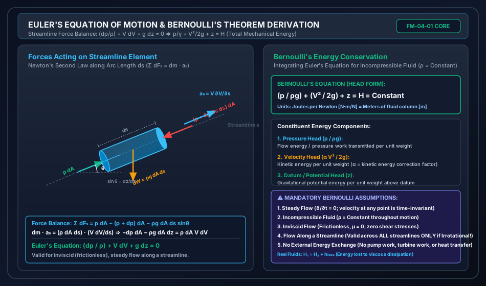
Applying Newton's second law along a curved streamline coordinate s balancing pressure forces, gravitational weight components, and convective acceleration yields the classical one-dimensional differential Euler equation:
Conservative Body Forces (gravity as the sole body force),
direct integration yields Bernoulli's Theorem:
ρgp+2gV2+z=H=Constant
where each term possesses the fundamental physical dimension of length [L], designated as Head (energy per unit weight, N⋅m/N=m):
γp=ρgp: Pressure Head (flow energy per unit weight transmitted across boundaries),
2gV2: Velocity Head (kinetic energy per unit weight),
z: Datum Head / Potential Head (gravitational potential energy per unit weight above an arbitrary datum).
Crucially:
Along a Streamline vs Across the Entire Flow Field: For rotational flow, the Bernoulli constant H varies from one streamline to another (H=H(ψ)). However, if the flow is strictly Irrotational (∇×V=0), the Bernoulli constant H is universally identical across all streamlines throughout the entire flow field.
Non-Uniform Velocity Profiles & Kinetic Energy Correction Factor (α): Real flows across conduits exhibit boundary-layer velocity gradients. To use the one-dimensional cross-sectional mean velocity V=Q/A in the energy equation, the true kinetic energy flux is corrected by the dimensionless factor α=AV31∫u3dA. For laminar flow in a circular pipe, α=2.0; for turbulent pipe flow, α≈1.03–1.06 (frequently taken as α≈1.0 in high-Reynolds engineering design).
Energy Grade Line (EGL / TEL) & Hydraulic Grade Line (HGL):
The Total Energy Line (EGL) plots the total mechanical energy head (z+γp+2gV2). For real fluids without mechanical energy inputs, the EGL must monotonically drop in the direction of flow at a slope equal to the friction slope Sf=−dEGL/dx. Pumps cause a vertical jump +Hp; turbines cause a vertical drop −Ht.
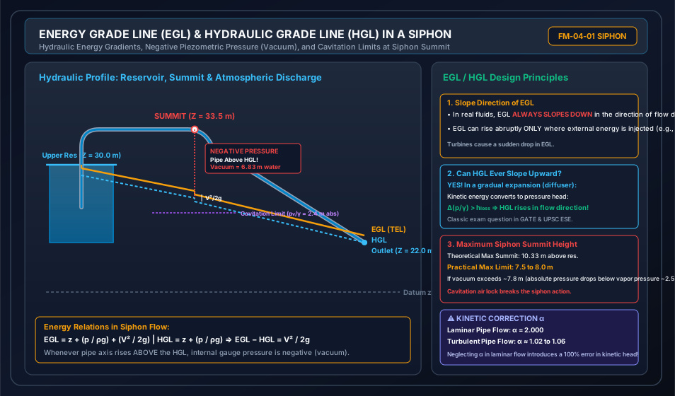
The Hydraulic Grade Line (HGL) plots the piezometric head (z+γp). The vertical gap between EGL and HGL is exactly the velocity head 2gV2. When a conduit rises above the HGL (such as at the summit of a siphon), the gauge pressure becomes negative (vacuum). If the absolute pressure plummets to the fluid vapor pressure (pvap/γ≈2.4 m of water absolute at 20∘C), dissolved gases violently de-aerate and water vapor pockets boil, precipitating destructive Cavitation and air-lock flow termination.
3. Forces Acting on Fluid Elements & Euler's Equation along a Streamline
3.1 Forces Governing Fluid Motion
In continuum fluid mechanics, Newton's second law for a moving fluid element states:
Fnet=ma=Fg+Fp+Fv+Ft+Fc+Fσ
where:
Fg: Gravity body force,
Fp: Pressure force (normal surface stresses),
Fv: Viscous shear force (tangential surface stresses due to molecular viscosity),
Ft: Reynolds turbulent shear force (apparent stresses due to turbulent momentum fluctuations),
Fc: Compressibility / elastic force (significant only when Mach number M>0.3),
Fσ: Surface tension force (significant only at interfaces with high curvature or micro-channels).
Hierarchy of dynamic equations:
Navier-Stokes Equations: Retains Fg+Fp+Fv. (Governs viscous laminar and DNS turbulent flow).
Euler's Equation: Retains only Gravity and Pressure forces (Fg+Fp). Viscous shear forces (Fv=0), turbulent stresses (Ft=0), and compressibility forces (Fc=0) are neglected.
3.2 Formal Derivation of Euler's Equation along a Streamline
Consider a small cylindrical fluid element of length ds and cross-sectional area dA moving along a streamline oriented at an angle θ to the horizontal. Let the vertical coordinate be z, such that the elevation difference over distance ds is:
sinθ=dsdz
           ^ s (Streamline direction)
          /
         /   [p - (dp/ds)*(ds/2)] * dA
        +-------------------------+
        |                         |
        |      Fluid Element      | ===> Flow velocity V
        |      Mass = rho*dA*ds   |
        |            |            |
        +------------|------------+
       /             v Weight dW = rho*g*dA*ds
      /
     / [p + (dp/ds)*(ds/2)] * dA
    +-----------------------------------> Horizontal x
     \ theta
Step 1: Mass of the Element
The volume of the cylindrical element is d∀=dA⋅ds. The elemental mass is:
dm=ρd∀=ρdAds
Step 2: Surface Forces Acting Parallel to the Streamline
Pressure acts perpendicularly on the two circular end faces:
Pressure force at upstream face s−2ds:
Fp1=(p−∂s∂p2ds)dA
Pressure force at downstream face s+2ds:
Fp2=−(p+∂s∂p2ds)dA
Net pressure force along s:
dFp=Fp1+Fp2=−∂s∂pdsdA
(Note: Pressure forces acting on the circumferential lateral mantle are perpendicular to the streamline s everywhere and thus exert zero component along s in an inviscid fluid).
Step 3: Body Force Acting Parallel to the Streamline
The total weight of the element acting vertically downwards is:
dW=dm⋅g=ρgdAds
The component of this gravitational weight opposing motion along the streamline (+s direction) is:
dFg=−dWsinθ=−ρgdAdssinθ
Substituting sinθ=dsdz:
dFg=−ρgdAds(dsdz)=−ρgdAdz
Step 4: Total Applied Force along the Streamline
∑dFs=dFp+dFg=−∂s∂pdsdA−ρgdAdz
Step 5: Acceleration along the Streamline
From fluid kinematics (Topic FM-03-03), the total particle acceleration along a streamline coordinate s is the substantial derivative:
as=DtDs=∂t∂V+V∂s∂V
For steady flow (∂t∂V=0):
as=V∂s∂V
Step 6: Equating via Newton's Second Law (∑dFs=dm⋅as)
−∂s∂pdsdA−ρgdAdz=(ρdAds)(V∂s∂V)
Divide the entire equation by the elemental mass ρdAds:
−ρ1∂s∂p−gdsdz=V∂s∂V
Rearranging all terms to one side and multiplying by ds (since flow is along the specific streamline path where variations occur solely with s):
ρdp+VdV+gdz=0
This fundamental differential relationship is Euler's Equation of Motion along a Streamline.
4. Integration to Bernoulli's Equation & The 5 Fundamental Assumptions
4.1 Integration along a Streamline
Integrating Euler's differential equation along the streamline:
∫ρdp+∫VdV+∫gdz=Constant
For an incompressible fluid (ρ=constant):
ρp+2V2+gz=C
Dividing throughout by the gravitational acceleration g (where specific weight γ=ρg):
ρgp+2gV2+z=H=Constant
This is Bernoulli's Equation.
4.2 The Five Essential Assumptions of Classical Bernoulli's Theorem
To prevent invalid application in engineering analysis, the five core assumptions must be strictly remembered:
Steady Flow: Flow variables (V,p,ρ) at any fixed spatial point do not vary with time (∂/∂t=0). Unsteady acceleration (∂V/∂t) is zero.
Incompressible Flow: Density ρ is constant throughout the motion. (For gases, valid only when Mach number M<0.3 and pressure variations Δp/p<0.05).
Frictionless / Inviscid Flow: Viscosity μ=0. Shear stresses τ=μdydu=0. Mechanical energy is not dissipated into thermal internal energy.
Flow along a Streamline: The energy balance applies between two points located on the same streamline.
Conservative Body Forces: Gravity is the sole active body force (no magnetic, electromagnetic, or centrifugal force fields outside natural gravity).
4.3 Extension: Bernoulli's Equation across the Entire Flow Field (Irrotational Flow)
Does the constant H remain equal between two different streamlines?
Consider the full vector form of Euler's equation for steady incompressible flow:
(V⋅∇)V=−ρ1∇p−g∇z
Using the vector identity (V⋅∇)V=∇(2V2)−V×(∇×V):
∇(2V2)−V×ζ=−∇(ρp+gz)
where ζ=∇×V=2ω is the vorticity vector. Rearranging:
∇(ρp+2V2+gz)=V×ζ
Taking the scalar dot product with an arbitrary displacement vector dr:
d(ρp+2V2+gz)=(V×ζ)⋅dr
Now examine two distinct cases:
Case 1: Displacement along a streamline (dr∥V)
The vector cross product (V×ζ) is perpendicular to V. Therefore:
(V×ζ)⋅dr=0⟹ρgp+2gV2+z=H(ψ)=Constant along that streamline
If the flow is rotational (ζ=0), H varies from streamline to streamline!
Case 2: Irrotational Flow (ζ=∇×V=0) everywhere
Then (V×ζ)≡0 in all directions. Thus:
∇(ρgp+2gV2+z)=0⟹ρgp+2gV2+z=H=Universal Constant Everywhere
Key Takeaway for GATE/ESE:
In rotational flow, Bernoulli's equation can ONLY be applied between two points on the same streamline.
In irrotational flow, Bernoulli's equation can be applied between ANY two points in the flow field, whether on the same streamline or on completely different streamlines.
4.4 Compressible Flow Bernoulli's Equation
When density is variable (ρ=ρ(p)), Euler's equation integrates to:
∫ρ(p)dp+2V2+gz=Constant
Isothermal Process (p/ρ=C1=RT=const):∫p/C1dp=C1lnp=ρplnp⟹ρ1p1lnp+2V2+gz=Constant
Adiabatic / Isentropic Process (p/ρk=C2 where k=Cp/Cv):∫(p/C2)1/kdp=k−1kρp⟹(k−1k)ρp+2V2+gz=Constant
5. Kinetic Energy Correction Factor (α) for Non-Uniform Velocity Distributions
In one-dimensional engineering pipe and open-channel hydraulics, calculations are performed using the bulk mean cross-sectional velocity:
Vavg=V=AQ=A1∫AudA
However, fluid shear at solid boundaries generates a non-uniform velocity distribution u(y) or u(r). The actual kinetic energy passing through an elemental area dA per unit time is:
d(KE˙)=21(dm)u2=21(ρudA)u2=21ρu3dA
Integrating over the entire cross-section A, the true rate of kinetic energy transmission is:
KE˙actual=21ρ∫Au3dA
If calculated naively using the average velocity V:
KE˙1D=21(ρAV)V2=21ρAV3
Because the cube of the average is always less than the average of the cubes (Cauchy-Schwarz / Jensen's Inequality), KE˙actual≥KE˙1D.
The Kinetic Energy Correction Factor (Coriolis Coefficient)α is defined as:
Accordingly, the true velocity head in the 1D Bernoulli equation is:
True Velocity Head=α2gV2
5.1 Analytical Derivation for Fully Developed Laminar Pipe Flow
For laminar flow in a circular pipe of radius R, the Hagen-Poiseuille parabolic velocity distribution is:
u(r)=Umax[1−(Rr)2]
The mean velocity is:
V=2Umax
Elemental area of a ring: dA=2πrdr. Cross-sectional area A=πR2.
Let dimensionless radius η=(r/R)2⟹dη=R22rdr⟹2πrdr=πR2dη.
Substitute into the definition of α:
6. Extended Energy Equation with Real Fluid Friction & External Work
Real fluids possess viscosity (μ>0). Viscous shear stresses within the fluid and at solid conduit boundaries dissipate mechanical energy into irreversible thermal energy, designated as Head Loss (hL). Furthermore, hydraulic systems often include mechanical turbomachinery:
Pumps: Add mechanical energy to the fluid (Pump Head, Hp).
Turbines: Extract mechanical energy from the fluid (Turbine Head, Ht).
The Extended 1D Engineering Energy Equation between section 1 (upstream) and section 2 (downstream) is:
Major Friction Loss (hf): Darcy-Weisbach equation hf=2gDfLV2.
Minor Local Losses (∑hm): Minor losses at fittings, bends, entrances, and expansions: ∑KL2gV2.
Hydraulic Power added by pump: Pp=ηpγQHp (where ηp is pump efficiency).
Hydraulic Power generated by turbine: Pt=γQHtηt (where ηt is turbine efficiency).
7. Energy Grade Line (EGL/TEL), Hydraulic Grade Line (HGL) & Siphon Dynamics
7.1 Definitions & Physical Signatures
Total Energy Line (TEL / EGL):
A graphical plot representing the total mechanical energy head per unit weight of fluid with respect to an arbitrary horizontal datum:
EGL=z+γp+2gV2
Hydraulic Grade Line (HGL):
A graphical plot representing the Piezometric Head (potential plus static pressure head):
HGL=z+γp
The HGL represents the height to which liquid would rise in a vertical piezometer tube inserted into the conduit at that location.
For open-channel flow where surface gauge pressure p=0, the HGL coincides exactly with the Free Liquid Surface.
7.2 Strict Geometric & Hydraulic Rules Governing EGL and HGL
Vertical Separation:EGL−HGL=2gV2=Velocity Head
The EGL is always strictly above the HGL by distance V2/(2g) for moving fluids.
The EGL can touch the HGL only at stagnation points where V=0 (e.g., inside large quiescent reservoirs).
In a constant-diameter pipe carrying steady incompressible flow (V=const), the velocity head is uniform; therefore, EGL and HGL are strictly parallel.
Directional Slope (Real Fluids):
For passive conduits without pumps, the EGL must continually slope downward in the direction of flow. The rate of drop represents energy dissipation:
Slope of EGL=Sf=−dxd(EGL)=LhL>0
The HGL can slope downward OR upward:
In an expanding conduit (diffuser), velocity decreases (V2<V1), converting dynamic kinetic head into static pressure head (Pressure Recovery). If the pressure rise Δ(p/γ) exceeds local friction loss, the HGL slopes upward in the flow direction!
Turbomachinery Jumps:
A Pump imparts energy to the fluid, causing an abrupt upward vertical step in both EGL and HGL of magnitude +Hp.
A Turbine extracts energy, causing an abrupt downward vertical step in both EGL and HGL of magnitude −Ht.
Exit Conditions:
When a pipe discharges freely into the atmosphere, the static gauge pressure at the outlet is zero (p2=0). Thus, the HGL terminates precisely at the centerline of the pipe exit.
When discharging into a submerged reservoir, the HGL matches the reservoir surface, and the entire velocity head V2/(2g) is dissipated into heat via turbulent mixing (hexit=1.02gV2).
Energy Grade Line (EGL)  o==================\
                          |  V^2 / 2g        \========= EGL
Hydraulic Grade Line (HGL) \------------------\
                            |  p / gamma       \------- HGL
Pipe Centerline              \~~~~~~~~~~~~~~~~~~\====== Pipe
                              |  z (Datum Head)
------------------------------+-------------------------------- Horizontal Datum
A Siphon is a bent closed conduit used to convey liquid from a higher-elevation reservoir to a lower-elevation discharge point across an intermediate summit or topographic ridge whose elevation rises above the free surface of the supply reservoir.
The Siphon Mechanism
The siphon must be fully primed (purged of air pockets) to establish continuous liquid continuity.
The driving head producing flow through the siphon is simply the difference in liquid levels between the supply reservoir and the discharge outlet:
Hnet=Zres,1−Zdischarge(The summit height has NO effect on the net driving head, only on the summit internal pressure!)
At the summit, the pipe elevation zsummit exceeds the total energy available at that point. Because the conduit centerline rises above the Hydraulic Grade Line (HGL):
γpsummit=HGLsummit−zsummit<0(Negative Gauge Pressure / Vacuum)
Cavitation Limits & Boiling Vapor Pressure
As the height of the summit above the upper reservoir increases, the vacuum intensifies.
Atmospheric pressure at sea level:
γpatm≈10.33 m of water absolute(101.325 kPa)
The vapor pressure of water at ambient temperature (20∘C) is:
pvap≈2.34 kPa⟹γpvap≈0.24 m to 2.4 m of water absolute(In field civil engineering practice, due to dissolved air release and turbulent fluctuations, the safe practical cavitation limit is taken as pabs,min/γ≈2.4 m to 2.5 m of water absolute, or a maximum vacuum gauge head of 10.33−2.5=7.83 m of water vacuum).
If the summit absolute pressure drops below this critical vapor threshold:
Liquid water spontaneously flashes into vapor pockets.
Dissolved air de-aerates out of solution to form expanding air locks.
The siphon air-locks, the liquid column breaks, and discharge stops completely.
If vapor bubbles are swept downstream into higher-pressure zones, they collapse violently with micro-jet velocities exceeding 1000 m/s and local shock pressures up to 1000 MPa, eroding pipe surfaces via pitting cavitation damage.
8. Visual Diagrams & Architectural Schematics
8.1 Euler's Streamline Element & Bernoulli Integration
The schematic below details the fluid element balance along an inclined streamline coordinate s, illustrating the interplay between pressure gradients, gravity vector components, and particle convective acceleration.
8.2 Energy Grade Line (EGL), Hydraulic Grade Line (HGL) & Siphon Mechanics
The following hydraulic schematic illustrates a long-distance siphon installation conveying water over an elevated crest, displaying the slopes of EGL and HGL, entry/friction/bend losses, summit vacuum generation, and the cavitation danger boundary.
9. Step-by-Step Numerical Problems with Complete Calculations
Problem 1: Inclined Tapering Conduit with Elevation & Kinetic Energy Conversion
Problem Statement:
A tapering non-uniform pipeline carries water (ρ=1000 kg/m3,γ=9810 N/m3) under steady flow at a volumetric discharge of Q=0.120 m3/s (120 L/s).
At inlet section 1: Pipe diameter D1=0.30 m, elevation z1=4.0 m above datum, and static pressure p1=250.0 kPa.
At outlet section 2: Pipe diameter D2=0.15 m, and elevation z2=1.5 m above datum.
Assuming frictionless flow (hL=0) and uniform velocity distribution (α1=α2=1.0), determine:
Technical Commentary:
Notice that even though the velocity head increased significantly from 0.15 m to 2.35 m (a kinetic head increase of 2.203 m), the elevation dropped by 2.50 m (4.0 m→1.5 m). The potential energy drop exceeded the kinetic energy gain, resulting in a net pressure increase from 250.0 kPa to 252.91 kPa!
Problem 2: Evaluation of Kinetic Energy Correction Factor (α)
Problem Statement:
A laminar oil flow in a circular conduit follows the exact parabolic velocity distribution u(r)=Umax[1−(r/R)2]. Prove mathematically that the kinetic energy correction factor is α=2.0000.
For turbulent flow in the same pipe, the velocity distribution is approximated by the power-law profile u(r)=Umax(1−r/R)1/7. Calculate the exact fraction and decimal value of α.
If an engineer mistakenly neglects α in a laminar pipe flow calculation where mean velocity V=2.50 m/s, calculate the percentage error in the computed velocity head.
Solution & Step-by-Step Calculation:
Step 1: Proof for Laminar Flow
Mean velocity V=Umax/2.
Step 3: Percentage Error in Velocity Head for Laminar Flow
Nominal Velocity Head (assuming α=1)=2gV2=2×9.812.52=0.31855 mTrue Velocity Head=α2gV2=2.0×0.31855=0.63710 mUnderestimation Error=TrueTrue−Nominal×100%=2.02.0−1.0×100%=50.0%
(Neglecting α in laminar flow underpredicts the kinetic energy by exactly 50%).
Problem 3: Siphon Hydraulics, Summit Vacuum, Hydraulic Grade Line & Cavitation Check
Problem Statement:
A commercial steel siphon pipeline of diameter D=150 mm (0.150 m) and total length L=80.0 m draws water from an upper reservoir whose water surface elevation is Zres=30.0 m and discharges freely into the atmosphere at an outlet elevation Zout=22.0 m.
The siphon summit is located at elevation Zsummit=33.5 m (3.5 m above the upper reservoir surface).
Length of pipe from the upper reservoir entrance to the summit: L1=25.0 m.
Friction factor f=0.020.
Minor loss coefficients: Sharp entrance Kent=0.50, summit bend Kbend=0.40. The pipe discharges freely at the exit (Kexit=1.0 kinetic head lost).
Atmospheric pressure head patm/γ=10.33 m of water.
Critical vapor pressure head of water at ambient temperature pvap/γ=2.40 m of water absolute.
Determine:
Velocity V of water in the siphon and the volumetric discharge Q in L/s,
Total head loss from the upper reservoir to the summit,
Gauge pressure head and absolute pressure head at the summit,
Whether the siphon is safe from cavitation,
Values of the Energy Grade Line (EGL) and Hydraulic Grade Line (HGL) at the summit.
Solution & Step-by-Step Calculation:
Step 1: Total Available Net Driving Head and Discharge
Apply the extended energy equation between the upper reservoir surface (section 0) and the free atmospheric discharge jet (section 2):
Zres+γp0+2gV02=Zout+γp2+2gV22+hL,total
Here, p0=p2=0 (atmospheric gauge), and V0≈0 (large reservoir surface).
Total head loss in the system:
Step 2: Head Losses from Reservoir to Summit (L1=25.0 m)
hL,summit=(Kent+DfL1+Kbend)2gV2DfL1=0.1500.020×25.0=0.1500.50=3.33333∑Ksummit=0.50+3.33333+0.40=4.23333hL,summit=4.23333×0.63660 m=2.69496 m≈2.6950 m
Step 3: Pressure at the Summit
Apply the energy equation between upper reservoir (0) and summit (S):
Zres+0+0=Zsummit+(γps)gauge+2gV2+hL,summit30.0=33.5+(γps)gauge+0.63660+2.69496(γps)gauge=30.0−33.5−0.63660−2.69496=−6.83156 m≈−6.8316 m
Vacuum at Summit:6.83 m of water vacuum.
Absolute Pressure Head at Summit:
(γps)abs=γpatm+(γps)gauge=10.33 m+(−6.83156 m)=3.49844 m≈3.4984 m absolute
Step 4: Cavitation Check
(γps)abs=3.4984 m>γpvap=2.40 m absolute
Because the internal pressure head (3.50 m) remains safely above the vapor pressure limit (2.40 m) by a margin of 1.10 m, no cavitation or vapor lock will occur. The siphon operates safely and continuously.
Step 5: EGL and HGL Elevations at the Summit
EGLsummit=Zres−hL,summit=30.0 m−2.69496 m=27.30504 m≈27.3050 mHGLsummit=EGLsummit−2gV2=27.30504−0.63660=26.66844 m≈26.6684 m
Notice:
(γps)gauge=HGLsummit−Zsummit=26.66844−33.5=−6.83156 m
(Perfect mathematical agreement verified across all energy equations).
10. High-Yield Exam Pitfalls, Traps & Shortcuts
The "Rotational Bernoulli" Trap (GATE CE):
Trap: A question describes a 2D forced vortex flow (V=ωrθ^) and asks whether Bernoulli's constant H is the same between points A(r1) and B(r2) on different radial streamlines.
Truth: Forced vortex flow has non-zero vorticity (ζ=2ω=0); it is rotational. Therefore, HA=HB. Bernoulli's equation CANNOT be applied across different streamlines in a forced vortex!
In contrast: Free vortex flow (Vθ=C/r) is irrotational (ζ=0); Bernoulli's equation CAN be applied between ANY two points throughout the entire field.
The "HGL Cannot Rise" Fallacy (UPSC ESE / SSC JE):
Trap: Assertion: "The Hydraulic Grade Line must always drop in the direction of real fluid flow because energy is lost to friction."
Truth: False! The Total Energy Line (EGL) must always drop in passive flow. The Hydraulic Grade Line (HGL) can rise if kinetic energy is converted to pressure head faster than friction dissipates energy (e.g., in a gradual pipe expansion / diffuser: Δ(p/γ)=2gV12−V22−hL>0).
Gauge vs Absolute Pressure Head in Siphons (State AE / RRB JE):
Trap: Solving for maximum siphon height using pgauge=2.4 m.
Truth:2.4 m is the absolute pressure head (pabs/γ). In gauge terms, this corresponds to −7.93 m of water gauge pressure (or 7.93 m vacuum). Always convert atmospheric pressure to absolute: pabs=patm+pgauge.
Kinetic Energy Factor α for Laminar vs Turbulent:
Laminar pipe flow: α=2.0 (Velocity head is doubled: True KE=2.0×2gV2).
Turbulent pipe flow: α≈1.05–1.06≈1.0.
Parallel plates laminar flow: α=54/35≈1.543.
Bernoulli for Gases (Compressibility Boundary):
Standard incompressible Bernoulli's equation is valid for air/gas flows only when the Mach number M=V/c≤0.30 (flow velocities below ≈100 m/s in atmospheric air), where density variation Δρ/ρ≤5%.
11. Multi-Exam Question Bank (GATE, ESE, SSC JE, State AE, RRB JE)
Question 1 (GATE CE — Numerical Answer Type)
Water flows through a horizontal nozzle of inlet diameter D1=200 mm and exit diameter D2=100 mm. The pressure at the inlet is 150 kPa gauge and the nozzle discharges freely to the atmosphere. Neglecting all losses (hL=0) and taking ρ=1000 kg/m3,g=9.81 m/s2, the discharge through the nozzle in L/s is:
Consider the following statements regarding the Bernoulli equation:
It represents the conservation of mechanical energy along a streamline for an inviscid fluid.
The constant in Bernoulli's equation is identical for all streamlines in an irrotational flow field.
The kinetic energy correction factor α is strictly greater than or equal to 1.0 for any non-uniform velocity distribution.
For steady compressible isentropic flow, Bernoulli's equation takes the form k−1kρp+2V2+gz=Constant.
Which of these statements are correct?
A) 1 and 2 only
B) 1, 2, and 3 only
C) 2, 3, and 4 only
D) 1, 2, 3, and 4
Detailed Solution:
Statement 1: Correct (derived by integrating Euler's equation along a streamline for inviscid flow).
Statement 2: Correct (V×(∇×V)=0 identically everywhere when flow is irrotational).
Statement 3: Correct (by Jensen's inequality, A1∫(u/V)3dA≥1.0, with equality holding solely for perfectly uniform velocity).
Statement 4: Correct (isentropic integration ∫dp/ρ=k−1kρp).
Correct Answer: D
Question 3 (SSC JE)
The vertical distance between the Energy Grade Line (EGL) and the Hydraulic Grade Line (HGL) at any point in a pipeline represents:
A) Datum head (z)
B) Pressure head (p/γ)
C) Velocity head (V2/2g)
D) Total friction loss (hf)
Detailed Solution:EGL=z+γp+2gV2 and HGL=z+γp.
Therefore, EGL−HGL=2gV2, which is the velocity head.
Correct Answer: C
Question 4 (State PSC AE)
In a laminar flow through a circular pipe of radius R, the kinetic energy correction factor α is equal to:
A)1.00
B)1.33
C)1.50
D)2.00
Detailed Solution:
For parabolic velocity profile u(r)=Umax[1−(r/R)2], integration yields α=AV31∫u3dA=2.00.
Correct Answer: D
Question 5 (RRB JE)
A siphon will cease to function (air-lock / column separation) when:
A) The outlet is lower than the inlet
B) The absolute pressure at the summit drops to the vapor pressure of the liquid
C) The pipe diameter is increased
D) The length of the siphon pipe is reduced
Detailed Solution:
When the absolute pressure at the summit plummets to the fluid vapor pressure, water begins boiling at room temperature, releasing dissolved air and vapor pockets that break the siphon column.
Correct Answer: B
12. Comprehensive Summary, Formula Cheatsheet & Academic References
Master Formula Cheatsheet
Euler’s Equation along a Streamline:Bernoulli’s Equation (Incompressible, Inviscid):Total Energy Line (EGL):Hydraulic Grade Line (HGL):Kinetic Energy Correction Factor:Extended Energy Equation:Siphon Net Driving Head:Summit Absolute Pressure Head:ρdp+VdV+gdz=0ρgp+2gV2+z=H=ConstantEGL=z+γp+α2gV2HGL=z+γp=EGL−α2gV2α=AV31∫Au3dA(Laminar Pipe: 2.0;Turbulent Pipe: ≈1.06)γp1+α12gV12+z1+Hp=γp2+α22gV22+z2+Ht+hLΔZ=Zres−Zdischarge=(1+Kent+DfL+∑Kminor)2gV2(γps)abs=γpatm−(Zs−Zres)−2gV2−hL,inlet→s≥γpvap≈2.4 m
Academic References & Standard Source Texts
White, F. M. (2016). Fluid Mechanics (8th ed.). McGraw-Hill Education. Chapter 3: Integral Relations for a Control Volume; Chapter 4: Differential Relations for Fluid Flow.
Streeter, V. L., Wylie, E. B., & Bedford, K. W. (1998). Fluid Mechanics (9th ed.). WCB/McGraw-Hill. Chapter 3: Linear Momentum and Bernoulli Equations.
Modi, P. N., & Seth, S. M. (2018). Hydraulics and Fluid Mechanics Including Hydraulics Machines (22nd ed.). Standard Book House, New Delhi. Chapter 6: Dynamics of Fluid Flow.
Rajput, R. K. (2020). A Textbook of Fluid Mechanics and Hydraulic Machines (7th ed.). S. Chand & Company Ltd. Chapter 6: Fluid Dynamics.
IS 2951 (Part 1 & 2): Methods of Measurement of Fluid Flow by Means of Venturi Meters and Orifice Plates. Bureau of Indian Standards, New Delhi.