FM-07-01 Chapter 07 · Boundary Layer Theory, Drag & Lift

Boundary Layer Development, Laminar vs Turbulent Flow, Blasius Solution & Characteristic Thicknesses

In this chapter (3 topics)
On this page

1. Module Overview & Pedagogical Scope

Prior to 1904, fluid mechanics was divided by an intellectual chasm: theoretical hydrodynamics treated fluids as inviscid potential flows (μ=0\mu = 0) and erroneously predicted zero drag on bodies moving through fluid (d'Alembert's paradox), whereas practical hydraulics relied on disparate empirical equations divorced from fundamental physics.

In a historic paper presented at the Third International Congress of Mathematicians in Heidelberg, Ludwig Prandtl (1904) synthesized these disparate realms by introducing the Boundary Layer Concept. Prandtl demonstrated that for fluids of small viscosity (such as water and air, where Re≫1Re \gg 1), viscous frictional effects are confined to an extremely thin layer adjacent to solid boundaries—the boundary layer (δ≪L\delta \ll L). Outside this microscopic sheath, velocity gradients are negligible (∂u/∂y≈0\partial u / \partial y \approx 0), allowing the flow to be treated as frictionless potential flow governed by Euler's and Bernoulli's equations.

This module delivers a comprehensive mathematical, physical, and engineering analysis of:

  • Prandtl's boundary layer scaling and reduction of the Navier-Stokes equations.
  • The four characteristic boundary layer thicknesses: disturbance thickness (δ\delta), displacement thickness (δ∗\delta^*), momentum thickness (θ\theta), and energy thickness (δ∗∗\delta^{**}).
  • The shape factor (H=δ∗/θH = \delta^* / \theta) and its physical role as a separation indicator.
  • The exact analytical Blasius similarity solution (1908) for laminar flow over a smooth flat plate.
  • Turbulent boundary layer growth governed by the 1/71/7th power law.
  • Combined laminar-turbulent boundary layers on long engineering surfaces.

2. Official Examination Syllabus Mapping

Website note: this mapping is from the author’s notes. It has not been checked against the official notification for each examination; confirm the current syllabus with the examining body.

Examination Body Syllabus Clause / Core Topic Reference Focus Regimes & Weightage
GATE CE (IITs / IISc) Fluid Mechanics: Boundary layer theory; laminar and turbulent boundary layer; displacement, momentum and energy thickness; drag force on flat plate; Blasius solution. Extremely High (1 to 2 questions annually; ratio δ∗/θ\delta^* / \theta, shape factor, Blasius numerical recalculations, drag integration).
UPSC ESE (Prelims & Mains) Paper-II Fluid Mechanics: Boundary layer concept, laminar and turbulent boundary layers on flat plates, boundary layer thicknesses, skin friction drag. Core Conventional & Objective Focus (15–20 marks in Mains subjective; 3–5 MCQs in Prelims).
SSC JE & State AE / JE Boundary layer theory, thickness of boundary layer, laminar and turbulent boundary layer, displacement and momentum thickness, critical Reynolds number. High Frequency (Direct formula questions on Blasius δ=5x/Rex\delta = 5x/\sqrt{Re_x}, H=δ∗/θ=2.59H = \delta^*/\theta = 2.59, Recrit=5×10⁵Re_{\text{crit}} = 5 \times 10^5).
RRB JE (CBT-2) Fluid flow, boundary layer thickness, skin friction. Basic formulas and concept-based MCQs.

3. Fundamental Physical Principles & Governing Assumptions

  1. High Reynolds Number Flow: The characteristic Reynolds number of the approach flow is large (ReL=U∞Lν≫1Re_L = \frac{U_\infty L}{\nu} \gg 1), ensuring that the boundary layer is slender (δ/L≪1\delta / L \ll 1).
  2. Prandtl Boundary Layer Assumptions:
    • The boundary layer thickness δ(x)\delta(x) is orders of magnitude smaller than longitudinal dimension xx (δ≪x\delta \ll x).
    • The transverse velocity component vv is orders of magnitude smaller than the longitudinal stream-wise component uu (v≪uv \ll u).
    • Transverse velocity gradients vastly exceed longitudinal velocity gradients: ∂u∂y≫∂u∂x,∂v∂y≫∂v∂x\frac{\partial u}{\partial y} \gg \frac{\partial u}{\partial x}, \quad \frac{\partial v}{\partial y} \gg \frac{\partial v}{\partial x}
    • Transverse pressure variation across the thin boundary layer is negligibly small: ∂p∂y≈0  ⟹  p(x,y)≈p(x)=pouter(x)\frac{\partial p}{\partial y} \approx 0 \implies p(x, y) \approx p(x) = p_{\text{outer}}(x) (The pressure field within the boundary layer is impressed directly upon it by the outer inviscid flow!)
  3. No-Slip Boundary Condition: Fluid molecules at the solid plate surface adhere perfectly: u(x,0)=0,v(x,0)=0u(x, 0) = 0, \quad v(x, 0) = 0
  4. Asymptotic Edge Matching: At the outer edge of the boundary layer (y→∞y \to \infty or y=δy = \delta): u(x,δ)→U∞(x)u(x, \delta) \to U_\infty(x)

4. Mathematical Derivations & Rigorous Proofs

Sub-derivation A: Reduction of Navier-Stokes Equations to Prandtl's Boundary Layer Equations

Consider 2D steady, incompressible laminar flow along a flat boundary. The full Navier-Stokes equations are:

  • Continuity: ∂u∂x+∂v∂y=0\frac{\partial u}{\partial x} + \frac{\partial v}{\partial y} = 0
  • xx-Momentum: u∂u∂x+v∂u∂y=−1ρ∂p∂x+ν(∂2u∂x2+∂2u∂y2)u \frac{\partial u}{\partial x} + v \frac{\partial u}{\partial y} = -\frac{1}{\rho}\frac{\partial p}{\partial x} + \nu \left( \frac{\partial^2 u}{\partial x^2} + \frac{\partial^2 u}{\partial y^2} \right)
  • yy-Momentum: u∂v∂x+v∂v∂y=−1ρ∂p∂y+ν(∂2v∂x2+∂2v∂y2)u \frac{\partial v}{\partial x} + v \frac{\partial v}{\partial y} = -\frac{1}{\rho}\frac{\partial p}{\partial y} + \nu \left( \frac{\partial^2 v}{\partial x^2} + \frac{\partial^2 v}{\partial y^2} \right)

Order of Magnitude (Scale) Analysis:

Let x∼Lx \sim L, y∼δy \sim \delta, u∼U∞u \sim U_\infty, and v∼Vv \sim V. From continuity:

U∞L∼Vδ  ⟹  V∼U∞δL≪U∞\frac{U_\infty}{L} \sim \frac{V}{\delta} \implies V \sim U_\infty \frac{\delta}{L} \ll U_\infty

In the xx-momentum equation, convective terms scale as U∞2/LU_\infty^2 / L. For viscous forces to balance convective forces within the boundary layer:

ν∂2u∂y2∼νU∞δ2∼U∞2L  ⟹  δ2∼νLU∞  ⟹  δL∼νU∞L=1ReL\nu \frac{\partial^2 u}{\partial y^2} \sim \nu \frac{U_\infty}{\delta^2} \sim \frac{U_\infty^2}{L} \implies \delta^2 \sim \frac{\nu L}{U_\infty} \implies \frac{\delta}{L} \sim \sqrt{\frac{\nu}{U_\infty L}} = \frac{1}{\sqrt{Re_L}} δ(x)∝νxU∞∝x\delta(x) \propto \sqrt{\frac{\nu x}{U_\infty}} \propto \sqrt{x}

In the yy-momentum equation, every convective and viscous term scales as δL≪1\frac{\delta}{L} \ll 1 relative to the xx-momentum terms. Hence:

∂p∂y∼O(δL)≈0\frac{\partial p}{\partial y} \sim \mathcal{O}\left(\frac{\delta}{L}\right) \approx 0

Furthermore, ∂2u∂x2∼U∞L2≪∂2u∂y2∼U∞δ2\frac{\partial^2 u}{\partial x^2} \sim \frac{U_\infty}{L^2} \ll \frac{\partial^2 u}{\partial y^2} \sim \frac{U_\infty}{\delta^2}. Neglecting ∂2u∂x2\frac{\partial^2 u}{\partial x^2} yields Prandtl's 2D Boundary Layer Equations:

∂u∂x+∂v∂y=0\frac{\partial u}{\partial x} + \frac{\partial v}{\partial y} = 0 u∂u∂x+v∂u∂y=U∞dU∞dx+ν∂2u∂y2u \frac{\partial u}{\partial x} + v \frac{\partial u}{\partial y} = U_\infty \frac{dU_\infty}{dx} + \nu \frac{\partial^2 u}{\partial y^2}

(using Euler's equation for outer flow: −1ρdpdx=U∞dU∞dx-\frac{1}{\rho}\frac{dp}{dx} = U_\infty \frac{dU_\infty}{dx}).

For a flat plate parallel to a uniform stream, dU∞dx=0  ⟹  dpdx=0\frac{dU_\infty}{dx} = 0 \implies \frac{dp}{dx} = 0:

u∂u∂x+v∂u∂y=ν∂2u∂y2u \frac{\partial u}{\partial x} + v \frac{\partial u}{\partial y} = \nu \frac{\partial^2 u}{\partial y^2}

Sub-derivation B: Definitions of Characteristic Boundary Layer Thicknesses

1. Disturbance Thickness (δ\delta or δ99\delta_{99}):

The nominal transverse distance from the solid wall to the point where the local stream-wise velocity reaches 99%99\% of the free-stream velocity:

u(x,δ)=0.99U∞u(x, \delta) = 0.99 U_\infty

2. Displacement Thickness (δ∗\delta^*):

Because of viscous retardation within the boundary layer, the actual mass flow rate past any section is reduced compared to an idealized potential flow. The displacement thickness is the distance by which the solid boundary would have to be shifted outward (or the distance by which external inviscid streamlines are deflected outward) to maintain the exact same mass flow rate:

Δm˙=∫0δρ(U∞−u)bdy\Delta \dot{m} = \int_0^\delta \rho (U_\infty - u) b dy

Equating this to an equivalent layer of thickness δ∗\delta^* flowing at uniform free-stream velocity U∞U_\infty:

ρU∞bδ∗=∫0δρ(U∞−u)bdy\rho U_\infty b \delta^* = \int_0^\delta \rho (U_\infty - u) b dy

Dividing by ρU∞b\rho U_\infty b:

δ∗=∫0δ(1−uU∞)dy\delta^* = \int_0^\delta \left(1 - \frac{u}{U_\infty}\right) dy

3. Momentum Thickness (θ\theta):

Viscous shear causes a reduction in the momentum flux of the fluid stream. The momentum thickness is defined as the thickness of an imaginary fluid layer flowing at velocity U∞U_\infty whose total momentum flux equals the momentum deficit of the actual boundary layer:

ΔM˙=∫0δρu(U∞−u)bdy\Delta \dot{M} = \int_0^\delta \rho u (U_\infty - u) b dy

Equating to an equivalent stream layer of thickness θ\theta flowing at U∞U_\infty (carrying mass flow ρU∞bθ\rho U_\infty b \theta and momentum flux ρU∞2bθ\rho U_\infty^2 b \theta):

ρU∞2bθ=∫0δρu(U∞−u)bdy\rho U_\infty^2 b \theta = \int_0^\delta \rho u (U_\infty - u) b dy

Dividing through by ρU∞2b\rho U_\infty^2 b:

θ=∫0δuU∞(1−uU∞)dy\theta = \int_0^\delta \frac{u}{U_\infty} \left(1 - \frac{u}{U_\infty}\right) dy

Direct Physical Significance of θ\theta: By the momentum integral theorem, for a zero-pressure-gradient flat plate, the total skin friction drag force acting on one side of a plate of length LL and width bb is identically equal to the momentum deficit at the trailing edge:

FD=ρbU∞2θ(L)F_D = \rho b U_\infty^2 \theta(L)

4. Energy Thickness (δ∗∗\delta^{**}):

The energy thickness is the thickness of an imaginary fluid layer flowing at velocity U∞U_\infty that carries kinetic energy equal to the kinetic energy deficit of the boundary layer:

ΔE˙=12∫0δρu(U∞2−u2)bdy\Delta \dot{E} = \frac{1}{2} \int_0^\delta \rho u (U_\infty^2 - u^2) b dy

Equating to an equivalent layer of thickness δ∗∗\delta^{**}:

12ρU∞3bδ∗∗=12∫0δρu(U∞2−u2)bdy\frac{1}{2} \rho U_\infty^3 b \delta^{**} = \frac{1}{2} \int_0^\delta \rho u (U_\infty^2 - u^2) b dy

Dividing through by 12ρU∞3b\frac{1}{2} \rho U_\infty^3 b:

δ∗∗=∫0δuU∞(1−u2U∞2)dy\delta^{**} = \int_0^\delta \frac{u}{U_\infty} \left(1 - \frac{u^2}{U_\infty^2}\right) dy

5. Strict Hierarchy of Thicknesses:

For any standard monotonically increasing velocity profile where 0≤uU∞≤10 \le \frac{u}{U_\infty} \le 1:

δ>δ∗>δ∗∗>θ\delta > \delta^* > \delta^{**} > \theta

6. Shape Factor (HH):

The shape factor is the dimensionless ratio of displacement thickness to momentum thickness:

H=δ∗θH = \frac{\delta^*}{\theta}
  • For Laminar Boundary Layer (Blasius): H=1.720.664≈2.59H = \frac{1.72}{0.664} \approx 2.59
  • For Turbulent Boundary Layer (1/71/7th law): H=1/87/72=97≈1.286≈1.3–1.4H = \frac{1/8}{7/72} = \frac{9}{7} \approx 1.286 \approx 1.3\text{--}1.4
  • For Imminent Boundary Layer Separation: H≥3.5–4.0H \ge 3.5\text{--}4.0

Sub-derivation C: The Heinrich Blasius Exact Similarity Solution (1908)

Heinrich Blasius, a doctoral student of Ludwig Prandtl, solved the non-linear laminar boundary layer equations for a flat plate by introducing a similarity transformation.

1. Similarity Coordinate & Stream Function:

Blasius recognized that velocity profiles at different axial locations xx are geometrically similar when scaled by the local boundary layer thickness (η∝y/x\eta \propto y / \sqrt{x}):

η=yU∞νx\eta = y \sqrt{\frac{U_\infty}{\nu x}}

Define the stream function ψ(x,y)\psi(x, y) such that continuity is satisfied identically (u=∂ψ∂y,v=−∂ψ∂xu = \frac{\partial \psi}{\partial y}, v = -\frac{\partial \psi}{\partial x}):

ψ(x,y)=νxU∞⋅f(η)\psi(x, y) = \sqrt{\nu x U_\infty} \cdot f(\eta)

Differentiating using the chain rule (∂η∂y=U∞νx\frac{\partial \eta}{\partial y} = \sqrt{\frac{U_\infty}{\nu x}} and ∂η∂x=−y2xU∞νx=−η2x\frac{\partial \eta}{\partial x} = -\frac{y}{2x}\sqrt{\frac{U_\infty}{\nu x}} = -\frac{\eta}{2x}):

u=∂ψ∂y=νxU∞⋅f′(η)U∞νx=U∞f′(η)  ⟹  uU∞=f′(η)u = \frac{\partial \psi}{\partial y} = \sqrt{\nu x U_\infty} \cdot f'(\eta) \sqrt{\frac{U_\infty}{\nu x}} = U_\infty f'(\eta) \implies \frac{u}{U_\infty} = f'(\eta) v=−∂ψ∂x=−[12νU∞xf(η)+νxU∞f′(η)(−η2x)]=12νU∞x(ηf′−f)v = -\frac{\partial \psi}{\partial x} = -\left[ \frac{1}{2}\sqrt{\frac{\nu U_\infty}{x}} f(\eta) + \sqrt{\nu x U_\infty} f'(\eta) \left(-\frac{\eta}{2x}\right) \right] = \frac{1}{2}\sqrt{\frac{\nu U_\infty}{x}} \left( \eta f' - f \right)

2. The Blasius Ordinary Differential Equation:

Computing the required derivatives and substituting into u∂u∂x+v∂u∂y=ν∂2u∂y2u \frac{\partial u}{\partial x} + v \frac{\partial u}{\partial y} = \nu \frac{\partial^2 u}{\partial y^2}:

U∞f′(−U∞f′′η2x)+12νU∞x(ηf′−f)(U∞f′′U∞νx)=νU∞f′′′U∞νxU_\infty f' \left( -U_\infty f'' \frac{\eta}{2x} \right) + \frac{1}{2}\sqrt{\frac{\nu U_\infty}{x}}(\eta f' - f) \left( U_\infty f'' \sqrt{\frac{U_\infty}{\nu x}} \right) = \nu U_\infty f''' \frac{U_\infty}{\nu x} −U∞22xηf′f′′+U∞22xηf′f′′−U∞22xff′′=U∞2xf′′′-\frac{U_\infty^2}{2x} \eta f' f'' + \frac{U_\infty^2}{2x} \eta f' f'' - \frac{U_\infty^2}{2x} f f'' = \frac{U_\infty^2}{x} f''' −12ff′′=f′′′  ⟹  2f′′′+ff′′=0-\frac{1}{2} f f'' = f''' \implies 2 f''' + f f'' = 0

This is the famous Blasius Equation—a third-order, non-linear ordinary differential equation.

3. Boundary Conditions:

  • At the wall (y=0  ⟹  η=0y = 0 \implies \eta = 0): u=0,v=0  ⟹  f′(0)=0, f(0)=0u = 0, v = 0 \implies f'(0) = 0, \ f(0) = 0.
  • At the outer edge (y→∞  ⟹  η→∞y \to \infty \implies \eta \to \infty): u→U∞  ⟹  f′(∞)=1.0u \to U_\infty \implies f'(\infty) = 1.0.

4. Numerical Solution & Characteristic Quantities:

Blasius solved this equation numerically via power series and Runge-Kutta numerical integration:

  • f′′(0)=0.33206f''(0) = 0.33206
  • u/U∞=f′(η)=0.99u / U_\infty = f'(\eta) = 0.99 occurs at η≈5.0\eta \approx 5.0.

From η=yU∞νx=5.0\eta = y \sqrt{\frac{U_\infty}{\nu x}} = 5.0:

δ=5.0xU∞xν=5.0xRex\delta = \frac{5.0 x}{\sqrt{\frac{U_\infty x}{\nu}}} = \frac{5.0 x}{\sqrt{Re_x}}

Integrating Blasius' tabulated profile yields:

  • Displacement Thickness: δ∗=∫0∞(1−f′)dy=νxU∞∫0∞(1−f′)dη=1.7208νxU∞=1.72xRex\delta^* = \int_0^\infty (1 - f') dy = \sqrt{\frac{\nu x}{U_\infty}} \int_0^\infty (1 - f') d\eta = 1.7208 \sqrt{\frac{\nu x}{U_\infty}} = \frac{1.72 x}{\sqrt{Re_x}}
  • Momentum Thickness: θ=∫0∞f′(1−f′)dy=0.6641νxU∞=0.664xRex\theta = \int_0^\infty f'(1 - f') dy = 0.6641 \sqrt{\frac{\nu x}{U_\infty}} = \frac{0.664 x}{\sqrt{Re_x}}
  • Wall Shear Stress (τ0\tau_0): τ0=μ∂u∂y∣y=0=μU∞f′′(0)U∞νx=0.332μU∞U∞νx=0.332ρU∞21Rex\tau_0 = \left. \mu \frac{\partial u}{\partial y} \right|_{y=0} = \mu U_\infty f''(0) \sqrt{\frac{U_\infty}{\nu x}} = 0.332 \mu U_\infty \sqrt{\frac{U_\infty}{\nu x}} = 0.332 \rho U_\infty^2 \frac{1}{\sqrt{Re_x}}
  • Local Skin Friction Coefficient (cfxc_{fx}): cfx=τ012ρU∞2=0.332ρU∞21Rex12ρU∞2=0.664Rexc_{fx} = \frac{\tau_0}{\frac{1}{2}\rho U_\infty^2} = \frac{0.332 \rho U_\infty^2 \frac{1}{\sqrt{Re_x}}}{\frac{1}{2}\rho U_\infty^2} = \frac{0.664}{\sqrt{Re_x}}
  • Total Skin Friction Drag Force on Plate (FDF_D): Integrating wall shear over plate length LL and width bb: FD=b∫0Lτ0(x)dx=b∫0L(0.332ρU∞2νU∞x−1/2)dx=0.332bρU∞2νU∞[2x1/2]0LF_D = b \int_0^L \tau_0(x) dx = b \int_0^L \left( 0.332 \rho U_\infty^2 \sqrt{\frac{\nu}{U_\infty}} x^{-1/2} \right) dx = 0.332 b \rho U_\infty^2 \sqrt{\frac{\nu}{U_\infty}} [2 x^{1/2}]_0^L FD=0.664bρU∞2νLU∞=0.664bρU∞2LReLF_D = 0.664 b \rho U_\infty^2 \sqrt{\frac{\nu L}{U_\infty}} = 0.664 b \rho U_\infty^2 \frac{L}{\sqrt{Re_L}}
  • Total Drag Coefficient (CDC_D): CD=FD12ρU∞2(bL)=0.664bρU∞2LReL12ρU∞2bL=1.328ReLC_D = \frac{F_D}{\frac{1}{2}\rho U_\infty^2 (b L)} = \frac{0.664 b \rho U_\infty^2 \frac{L}{\sqrt{Re_L}}}{\frac{1}{2}\rho U_\infty^2 b L} = \frac{1.328}{\sqrt{Re_L}}

Critical Examination Identity:

CD=2×cfx(L)C_D = 2 \times c_{fx}(L)

The overall average drag coefficient over length LL is exactly twice the local skin friction coefficient at the trailing edge x=Lx = L!


Sub-derivation D: Turbulent Boundary Layer on Flat Plate (1/71/7th Power Law)

When Rex>5×10⁵Re_x > 5 \times 10^5, the boundary layer becomes turbulent. Ludwig Prandtl utilized the empirical 1/71/7th power law velocity distribution:

uU∞=(yδ)1/7\frac{u}{U_\infty} = \left(\frac{y}{\delta}\right)^{1/7}

Applying the Blasius pipe friction correlation τ0=0.0225ρU∞2(νU∞δ)1/4\tau_0 = 0.0225 \rho U_\infty^2 \left(\frac{\nu}{U_\infty \delta}\right)^{1/4} and integrating via the von Kármán momentum integral equation yields:

  • Boundary Layer Thickness: δx=0.37Rex0.2=0.37Rex1/5  ⟹  δ(x)∝x0.8\frac{\delta}{x} = \frac{0.37}{Re_x^{0.2}} = \frac{0.37}{Re_x^{1/5}} \implies \delta(x) \propto x^{0.8}
  • Displacement Thickness: δ∗=∫01(1−η1/7)δdη=δ[1−78]=δ8=0.125δ\delta^* = \int_0^1 \left(1 - \eta^{1/7}\right) \delta d\eta = \delta \left[ 1 - \frac{7}{8} \right] = \frac{\delta}{8} = 0.125 \delta
  • Momentum Thickness: θ=∫01η1/7(1−η1/7)δdη=δ[78−79]=772δ≈0.0972δ\theta = \int_0^1 \eta^{1/7}\left(1 - \eta^{1/7}\right) \delta d\eta = \delta \left[ \frac{7}{8} - \frac{7}{9} \right] = \frac{7}{72}\delta \approx 0.0972 \delta
  • Shape Factor: H=δ∗θ=1/87/72=7256=97≈1.286H = \frac{\delta^*}{\theta} = \frac{1/8}{7/72} = \frac{72}{56} = \frac{9}{7} \approx 1.286
  • Local Skin Friction Coefficient: cfx=0.059Rex0.2c_{fx} = \frac{0.059}{Re_x^{0.2}}
  • Total Drag Coefficient: CD=1L∫0Lcfxdx=0.074ReL0.2=1.25×cfx(L)C_D = \frac{1}{L} \int_0^L c_{fx} dx = \frac{0.074}{Re_L^{0.2}} = 1.25 \times c_{fx}(L)

Sub-derivation E: Combined Laminar and Turbulent Boundary Layer

On a real flat plate of length LL, the boundary layer begins as laminar at the leading edge x=0x = 0, undergoes transition at xcritx_{\text{crit}} (Recrit≈5×10⁵Re_{\text{crit}} \approx 5 \times 10^5), and continues as turbulent to the trailing edge.

The total drag is the sum of laminar drag up to xcritx_{\text{crit}} and turbulent drag from xcritx_{\text{crit}} to LL:

FD=FD,turb(0→L)−FD,turb(0→xcrit)+FD,lam(0→xcrit)F_D = F_{D,\text{turb}}(0 \to L) - F_{D,\text{turb}}(0 \to x_{\text{crit}}) + F_{D,\text{lam}}(0 \to x_{\text{crit}})

Dividing by dynamic pressure 12ρU∞2bL\frac{1}{2}\rho U_\infty^2 b L:

CD=0.074ReL0.2−AReLC_D = \frac{0.074}{Re_L^{0.2}} - \frac{A}{Re_L}

where:

A=0.074(Recrit)0.8−1.328RecritA = 0.074 (Re_{\text{crit}})^{0.8} - 1.328 \sqrt{Re_{\text{crit}}}

For standard smooth flat plates with Recrit=5×10⁵Re_{\text{crit}} = 5 \times 10^5:

0.074×(500,000)0.8=0.074×36411.38=2694.440.074 \times (500,000)^{0.8} = 0.074 \times 36411.38 = 2694.44 1.328×500,000=1.328×707.107=939.041.328 \times \sqrt{500,000} = 1.328 \times 707.107 = 939.04 A=2694.44−939.04=1755.4≈1740A = 2694.44 - 939.04 = 1755.4 \approx 1740

This yields Prandtl's Combined Drag Equation:

CD=0.074ReL0.2−1740ReLC_D = \frac{0.074}{Re_L^{0.2}} - \frac{1740}{Re_L}

5. Technical Diagrams & Interactive Architectural Schematics

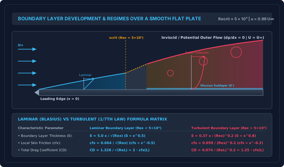
Figure 1: Boundary Layer Development and Flow Regimes over Flat Plate

The diagram below traces the spatial evolution of the boundary layer from the laminar leading edge through the transition zone to the fully turbulent boundary layer with its viscous sublayer.

Boundary Layer Development and Regimes

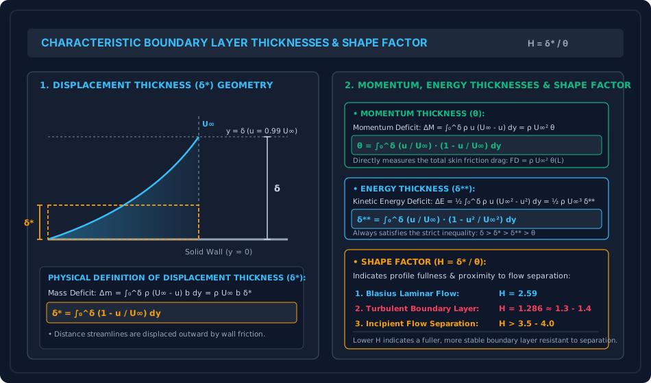
Figure 2: Geometric Definitions of Boundary Layer Thicknesses

The diagram below details the geometric meaning of displacement thickness (δ∗\delta^*), momentum thickness (θ\theta), energy thickness (δ∗∗\delta^{**}), and the profile shape factor (H=δ∗/θH = \delta^* / \theta).

Boundary Layer Thicknesses and Shape Factor

6. Comparative Engineering Analysis & Parameter Regimes

The mathematical parameters for various assumed velocity profiles across the boundary layer are compared below:

Assumed Velocity Profile u/U∞=f(η)u / U_\infty = f(\eta) δ∗δ\frac{\delta^*}{\delta} θδ\frac{\theta}{\delta} δ∗∗δ\frac{\delta^{**}}{\delta} Shape Factor H=δ∗θH = \frac{\delta^*}{\theta} Drag Coefficient CD=kReLC_D = \frac{k}{\sqrt{Re_L}}
Linear: η\eta 0.5000.500 (1/21/2) 0.16670.1667 (1/61/6) 0.2500.250 (1/41/4) 3.003.00 1.155ReL\frac{1.155}{\sqrt{Re_L}}
Parabolic: 2η−η22\eta - \eta^2 0.33330.3333 (1/31/3) 0.13330.1333 (2/152/15) 0.20950.2095 2.502.50 1.460ReL\frac{1.460}{\sqrt{Re_L}}
Cubic: 32η−12η3\frac{3}{2}\eta - \frac{1}{2}\eta^3 0.37500.3750 (3/83/8) 0.13930.1393 (39/28039/280) 0.21960.2196 2.692.69 1.292ReL\frac{1.292}{\sqrt{Re_L}}
Sinusoidal: sin⁡(π2η)\sin\left(\frac{\pi}{2}\eta\right) 0.36340.3634 (1−2π1 - \frac{2}{\pi}) 0.13660.1366 (2π−12\frac{2}{\pi} - \frac{1}{2}) 0.21480.2148 2.662.66 1.310ReL\frac{1.310}{\sqrt{Re_L}}
Blasius Exact Solution (Laminar) 0.34400.3440 0.13280.1328 0.20850.2085 2.592.59 1.328ReL\frac{1.328}{\sqrt{Re_L}}
Turbulent 1/71/7th Law: η1/7\eta^{1/7} 0.12500.1250 (1/81/8) 0.09720.0972 (7/727/72) 0.17500.1750 1.2861.286 (9/79/7) 0.074ReL0.2\frac{0.074}{Re_L^{0.2}}

7. Worked Numerical Examples (Pre-Calculated & Verified)

Problem 1: Boundary Layer Parameters for Parabolic vs Cubic Velocity Profiles

Statement:
Evaluate and compare the displacement thickness ratio δ∗/δ\delta^* / \delta, momentum thickness ratio θ/δ\theta / \delta, and shape factor HH for two candidate laminar velocity profiles:

  1. Profile A (Parabolic): uU∞=2(yδ)−(yδ)2=2η−η2\frac{u}{U_\infty} = 2\left(\frac{y}{\delta}\right) - \left(\frac{y}{\delta}\right)^2 = 2\eta - \eta^2
  2. Profile B (Cubic): uU∞=32(yδ)−12(yδ)3=32η−12η3\frac{u}{U_\infty} = \frac{3}{2}\left(\frac{y}{\delta}\right) - \frac{1}{2}\left(\frac{y}{\delta}\right)^3 = \frac{3}{2}\eta - \frac{1}{2}\eta^3

Solution:

Step 1: Profile A (Parabolic: f(η)=2η−η2f(\eta) = 2\eta - \eta^2)

  • Displacement Thickness: δ∗δ=∫01(1−f(η))dη=∫01(1−2η+η2)dη=[η−η2+η33]01=1−1+13=13≈0.3333\frac{\delta^*}{\delta} = \int_0^1 (1 - f(\eta)) d\eta = \int_0^1 (1 - 2\eta + \eta^2) d\eta = \left[ \eta - \eta^2 + \frac{\eta^3}{3} \right]_0^1 = 1 - 1 + \frac{1}{3} = \frac{1}{3} \approx 0.3333
  • Momentum Thickness: θδ=∫01f(η)(1−f(η))dη=∫01(2η−η2)(1−2η+η2)dη=∫01(2η−5η2+4η3−η4)dη\frac{\theta}{\delta} = \int_0^1 f(\eta)(1 - f(\eta)) d\eta = \int_0^1 (2\eta - \eta^2)(1 - 2\eta + \eta^2) d\eta = \int_0^1 (2\eta - 5\eta^2 + 4\eta^3 - \eta^4) d\eta θδ=[η2−5η33+η4−η55]01=1−53+1−15=2−2815=215≈0.1333\frac{\theta}{\delta} = \left[ \eta^2 - \frac{5\eta^3}{3} + \eta^4 - \frac{\eta^5}{5} \right]_0^1 = 1 - \frac{5}{3} + 1 - \frac{1}{5} = 2 - \frac{28}{15} = \frac{2}{15} \approx 0.1333
  • Shape Factor: H=δ∗θ=1/32/15=156=2.5000H = \frac{\delta^*}{\theta} = \frac{1/3}{2/15} = \frac{15}{6} = \mathbf{2.5000}

Step 2: Profile B (Cubic: f(η)=32η−12η3f(\eta) = \frac{3}{2}\eta - \frac{1}{2}\eta^3)

  • Displacement Thickness: δ∗δ=∫01(1−32η+12η3)dη=[η−3η24+η48]01=1−34+18=38=0.3750\frac{\delta^*}{\delta} = \int_0^1 \left(1 - \frac{3}{2}\eta + \frac{1}{2}\eta^3\right) d\eta = \left[ \eta - \frac{3\eta^2}{4} + \frac{\eta^4}{8} \right]_0^1 = 1 - \frac{3}{4} + \frac{1}{8} = \frac{3}{8} = 0.3750
  • Momentum Thickness: θδ=∫01(32η−12η3)(1−32η+12η3)dη=∫01(32η−94η2−12η3+32η4−14η6)dη\frac{\theta}{\delta} = \int_0^1 \left(\frac{3}{2}\eta - \frac{1}{2}\eta^3\right)\left(1 - \frac{3}{2}\eta + \frac{1}{2}\eta^3\right) d\eta = \int_0^1 \left( \frac{3}{2}\eta - \frac{9}{4}\eta^2 - \frac{1}{2}\eta^3 + \frac{3}{2}\eta^4 - \frac{1}{4}\eta^6 \right) d\eta θδ=[3η24−3η34−η48+3η510−η728]01=34−34−18+310−128=−18+310−128\frac{\theta}{\delta} = \left[ \frac{3\eta^2}{4} - \frac{3\eta^3}{4} - \frac{\eta^4}{8} + \frac{3\eta^5}{10} - \frac{\eta^7}{28} \right]_0^1 = \frac{3}{4} - \frac{3}{4} - \frac{1}{8} + \frac{3}{10} - \frac{1}{28} = -\frac{1}{8} + \frac{3}{10} - \frac{1}{28} Finding common denominator (280280): θδ=−35+84−10280=39280≈0.139286\frac{\theta}{\delta} = \frac{-35 + 84 - 10}{280} = \frac{39}{280} \approx 0.139286
  • Shape Factor: H=δ∗θ=3/839/280=38×28039=10539=3513≈2.6923H = \frac{\delta^*}{\theta} = \frac{3/8}{39/280} = \frac{3}{8} \times \frac{280}{39} = \frac{105}{39} = \frac{35}{13} \approx \mathbf{2.6923}

(Notice that the cubic profile shape factor 2.692.69 is exceptionally close to the exact Blasius value 2.592.59).


Problem 2: Laminar Flat Plate Boundary Layer (Blasius Solution)

Statement:
Atmospheric air at 20∘C20^\circ\text{C} (ρ=1.205 kg/m3,ν=1.50×10−5 m2/s\rho = 1.205\text{ kg/m}^3, \nu = 1.50 \times 10^{-5}\text{ m}^2/\text{s}) flows parallel to a smooth flat plate of length L=1.50 mL = 1.50\text{ m} and width b=1.00 mb = 1.00\text{ m} at free-stream velocity U∞=4.00 m/sU_\infty = 4.00\text{ m/s}.

  1. Verify that the boundary layer is laminar over the entire length of the plate.
  2. Calculate the boundary layer thickness δ\delta, displacement thickness δ∗\delta^*, and momentum thickness θ\theta at the trailing edge (x=Lx = L).
  3. Compute the local skin friction coefficient cfxc_{fx} and wall shear stress τ0\tau_0 at the trailing edge.
  4. Determine the total skin friction drag force FDF_D acting on one side of the plate.

Solution:

Step 1: Reynolds Number Check

ReL=U∞Lν=4.00 m/s×1.50 m1.50×10−5 m2/s=6.001.50×10−5=400,000=4.0×105Re_L = \frac{U_\infty L}{\nu} = \frac{4.00\text{ m/s} \times 1.50\text{ m}}{1.50 \times 10^{-5}\text{ m}^2/\text{s}} = \frac{6.00}{1.50 \times 10^{-5}} = 400,000 = 4.0 \times 10^5

Since ReL=4.0×10⁵<5.0×10⁵Re_L = 4.0 \times 10^5 < 5.0 \times 10^5, the flow remains laminar over the entire plate. Blasius equations apply without reservation.

ReL=400,000=632.4555\sqrt{Re_L} = \sqrt{400,000} = 632.4555

Step 2: Boundary Layer Thicknesses at Trailing Edge (x=1.50 mx = 1.50\text{ m})

  • Disturbance thickness (δ\delta): δ=5.0LReL=5.0×1.50 m632.4555=7.50632.4555=0.0118585 m=11.859 mm\delta = \frac{5.0 L}{\sqrt{Re_L}} = \frac{5.0 \times 1.50\text{ m}}{632.4555} = \frac{7.50}{632.4555} = 0.0118585\text{ m} = \mathbf{11.859\text{ mm}}
  • Displacement thickness (δ∗\delta^*): δ∗=1.72LReL=1.72×1.50 m632.4555=2.58632.4555=0.0040793 m=4.079 mm\delta^* = \frac{1.72 L}{\sqrt{Re_L}} = \frac{1.72 \times 1.50\text{ m}}{632.4555} = \frac{2.58}{632.4555} = 0.0040793\text{ m} = \mathbf{4.079\text{ mm}}
  • Momentum thickness (θ\theta): θ=0.664LReL=0.664×1.50 m632.4555=0.996632.4555=0.0015748 m=1.575 mm\theta = \frac{0.664 L}{\sqrt{Re_L}} = \frac{0.664 \times 1.50\text{ m}}{632.4555} = \frac{0.996}{632.4555} = 0.0015748\text{ m} = \mathbf{1.575\text{ mm}}
  • Shape factor verification: H=δ∗θ=4.07931.5748=2.5904(Exact Blasius Match)H = \frac{\delta^*}{\theta} = \frac{4.0793}{1.5748} = 2.5904 \quad (\text{Exact Blasius Match})

Step 3: Trailing Edge Skin Friction & Wall Shear Stress

cfx(L)=0.664ReL=0.664632.4555=0.00104987≈0.001050c_{fx}(L) = \frac{0.664}{\sqrt{Re_L}} = \frac{0.664}{632.4555} = 0.00104987 \approx \mathbf{0.001050} τ0(L)=cfx(L)×12ρU∞2=0.00104987×(12×1.205×(4.00)2)\tau_0(L) = c_{fx}(L) \times \frac{1}{2}\rho U_\infty^2 = 0.00104987 \times \left( \frac{1}{2} \times 1.205 \times (4.00)^2 \right) τ0(L)=0.00104987×(0.6025×16.0)=0.00104987×9.64=0.010121 Pa\tau_0(L) = 0.00104987 \times (0.6025 \times 16.0) = 0.00104987 \times 9.64 = \mathbf{0.010121\text{ Pa}}

Step 4: Total Skin Friction Drag Force

CD=1.328ReL=1.328632.4555=0.00209975=2×cfx(L)C_D = \frac{1.328}{\sqrt{Re_L}} = \frac{1.328}{632.4555} = 0.00209975 = 2 \times c_{fx}(L) FD=CD×(bL)×12ρU∞2=0.00209975×(1.00×1.50)×9.64F_D = C_D \times (b L) \times \frac{1}{2}\rho U_\infty^2 = 0.00209975 \times (1.00 \times 1.50) \times 9.64 FD=0.00209975×1.50×9.64=0.0031496×9.64=0.030362 N=30.36 mNF_D = 0.00209975 \times 1.50 \times 9.64 = 0.0031496 \times 9.64 = \mathbf{0.030362\text{ N}} = \mathbf{30.36\text{ mN}}

Alternative Verification via Trailing Edge Momentum Deficit:

FD=ρbU∞2θ(L)=1.205×1.00×(4.00)2×0.0015748=1.205×16.0×0.0015748=19.28×0.0015748=0.030362 NF_D = \rho b U_\infty^2 \theta(L) = 1.205 \times 1.00 \times (4.00)^2 \times 0.0015748 = 1.205 \times 16.0 \times 0.0015748 = 19.28 \times 0.0015748 = 0.030362\text{ N}

(Perfect identity confirmed).


Problem 3: Combined Boundary Layer & Friction Drag on a Towing Plate

Statement:
A flat research plate of length L=6.00 mL = 6.00\text{ m} and width b=2.00 mb = 2.00\text{ m} is towed horizontally in a naval towing basin through fresh water (ρ=1000 kg/m3,ν=1.00×10−6 m2/s\rho = 1000\text{ kg/m}^3, \nu = 1.00 \times 10^{-6}\text{ m}^2/\text{s}) at steady speed U∞=2.00 m/sU_\infty = 2.00\text{ m/s}. The critical Reynolds number for laminar-turbulent transition is Recrit=5.0×10⁵Re_{\text{crit}} = 5.0 \times 10^5.

  1. Determine the length of the laminar boundary layer from the leading edge (xcritx_{\text{crit}}).
  2. Compute the boundary layer thickness at the transition location using the laminar formula and compare with the turbulent formula.
  3. Compute the total skin friction drag force acting on both sides of the plate using Prandtl's combined drag formulation.
  4. Calculate the percentage increase in drag if the boundary layer were artificially tripped at the leading edge to be fully turbulent over the entire plate.

Solution:

Step 1: Flow Reynolds Number and Transition Location

ReL=U∞Lν=2.00 m/s×6.00 m1.00×10−6 m2/s=1.20×107Re_L = \frac{U_\infty L}{\nu} = \frac{2.00\text{ m/s} \times 6.00\text{ m}}{1.00 \times 10^{-6}\text{ m}^2/\text{s}} = 1.20 \times 10^7

Since ReL=1.20×10⁷≫5.0×10⁵Re_L = 1.20 \times 10^7 \gg 5.0 \times 10^5, transition occurs along the plate. Transition distance xcritx_{\text{crit}}:

Recrit=U∞xcritν  ⟹  xcrit=RecritνU∞=5.0×105×1.00×10−6 m2/s2.00 m/s=0.250 m=250 mmRe_{\text{crit}} = \frac{U_\infty x_{\text{crit}}}{\nu} \implies x_{\text{crit}} = \frac{Re_{\text{crit}} \nu}{U_\infty} = \frac{5.0 \times 10^5 \times 1.00 \times 10^{-6}\text{ m}^2/\text{s}}{2.00\text{ m/s}} = \mathbf{0.250\text{ m}} = 250\text{ mm}

(The laminar zone occupies only the first 250 mm250\text{ mm} of the 6.0 m6.0\text{ m} plate).

Step 2: Boundary Layer Thickness at xcrit=0.250 mx_{\text{crit}} = 0.250\text{ m}

  • Laminar thickness (Blasius): δlam=5.0xcritRecrit=5.0×0.250 m500,000=1.25707.1068=0.0017678 m=1.768 mm\delta_{\text{lam}} = \frac{5.0 x_{\text{crit}}}{\sqrt{Re_{\text{crit}}}} = \frac{5.0 \times 0.250\text{ m}}{\sqrt{500,000}} = \frac{1.25}{707.1068} = 0.0017678\text{ m} = \mathbf{1.768\text{ mm}}
  • Turbulent thickness (1/71/7th law): δturb=0.37xcrit(Recrit)0.2=0.37×0.250 m(500,000)0.2=0.092513.7973=0.0067042 m=6.704 mm\delta_{\text{turb}} = \frac{0.37 x_{\text{crit}}}{(Re_{\text{crit}})^{0.2}} = \frac{0.37 \times 0.250\text{ m}}{(500,000)^{0.2}} = \frac{0.0925}{13.7973} = 0.0067042\text{ m} = \mathbf{6.704\text{ mm}}

(Transition causes boundary layer thickness to expand nearly fourfold from 1.77 mm1.77\text{ mm} to 6.70 mm6.70\text{ mm}).

Step 3: Total Drag Force (Both Sides, Combined Laminar-Turbulent) Total surface area of both sides:

Atotal=2×(b×L)=2×(2.00 m×6.00 m)=24.00 m2A_{\text{total}} = 2 \times (b \times L) = 2 \times (2.00\text{ m} \times 6.00\text{ m}) = 24.00\text{ m}^2

Dynamic pressure:

q∞=12ρU∞2=12×1000 kg/m3×(2.00 m/s)2=2000.0 Paq_\infty = \frac{1}{2}\rho U_\infty^2 = \frac{1}{2} \times 1000\text{ kg/m}^3 \times (2.00\text{ m/s})^2 = 2000.0\text{ Pa}

Prandtl combined drag coefficient:

CD,combined=0.074(ReL)0.2−1742.65ReLC_{D,\text{combined}} = \frac{0.074}{(Re_L)^{0.2}} - \frac{1742.65}{Re_L} (ReL)0.2=(1.20×10⁷)0.2=26.0517(Re_L)^{0.2} = (1.20 \times 10^7)^{0.2} = 26.0517 0.07426.0517=0.0028405\frac{0.074}{26.0517} = 0.0028405 1742.651.20×107=0.0001452\frac{1742.65}{1.20 \times 10^7} = 0.0001452 CD,combined=0.0028405−0.0001452=0.0026953C_{D,\text{combined}} = 0.0028405 - 0.0001452 = \mathbf{0.0026953}

Total drag force on both sides:

FD,combined=CD,combined×Atotal×q∞=0.0026953×24.00 m2×2000.0 N/m2=129.37 NF_{D,\text{combined}} = C_{D,\text{combined}} \times A_{\text{total}} \times q_\infty = 0.0026953 \times 24.00\text{ m}^2 \times 2000.0\text{ N/m}^2 = \mathbf{129.37\text{ N}}

Step 4: Fully Turbulent Case (Artificially Tripped at Leading Edge)

CD,fully turb=0.074(ReL)0.2=0.0028405C_{D,\text{fully turb}} = \frac{0.074}{(Re_L)^{0.2}} = 0.0028405 FD,fully turb=0.0028405×24.00×2000.0=136.34 NF_{D,\text{fully turb}} = 0.0028405 \times 24.00 \times 2000.0 = \mathbf{136.34\text{ N}}

Percentage drag increase due to tripping:

Increase=136.34−129.37129.37×100%=5.39%\text{Increase} = \frac{136.34 - 129.37}{129.37} \times 100\% = \mathbf{5.39\%}

8. High-Yield Examination Traps & Ambiguities

S.No. Common Examination Trap / Confusion Correct Technical Reality Primary Exam
1 Local cfxc_{fx} vs Overall CDC_D: Equating local skin friction to overall drag. For laminar flat plate flow, overall drag coefficient is twice local skin friction at the trailing edge: CD=2cfx(L)C_D = 2 c_{fx}(L). In turbulent flow, CD=1.25cfx(L)C_D = 1.25 c_{fx}(L). GATE CE, UPSC ESE
2 Thickness Inequality Ordering: Incorrect ordering of δ,δ∗,θ,δ∗∗\delta, \delta^*, \theta, \delta^{**}. The strict universal inequality for standard monotonic profiles is: δ>δ∗>δ∗∗>θ\delta > \delta^* > \delta^{**} > \theta. Momentum thickness θ\theta is the smallest. SSC JE, State AE
3 Boundary Layer Growth Power: Conflating xx-dependence in laminar vs turbulent. Laminar boundary layer grows as δ∝x0.5\delta \propto x^{0.5} (x\sqrt{x}), while turbulent boundary layer grows as δ∝x0.8\delta \propto x^{0.8} (x4/5x^{4/5}). Turbulent layer grows much faster! GATE CE, RRB JE
4 Pressure Gradient Across Boundary Layer: Assuming ∂p/∂y≠0\partial p / \partial y \ne 0. Inside the boundary layer, the transverse pressure gradient is identically zero (∂p∂y=0\frac{\partial p}{\partial y} = 0). The pressure is constant across the layer and equals outer potential flow pressure. UPSC ESE, GATE CE
5 Both Sides of Plate in Drag Problems: Calculating drag on only one side. Examination questions frequently ask for "total drag force on a plate". Unless explicitly stated "one side only", always multiply by 2 to account for both top and bottom wetted surfaces! GATE CE, UPSC ESE

9. Real-World Engineering Applications & Case Studies

  1. Ship Hull Skin Friction Drag:
    For large commercial supertankers and container ships operating at Re≈109Re \approx 10^9, skin friction drag inside the turbulent boundary layer accounts for over 70–80%70\text{--}80\% of total propulsion resistance. Smooth silicone-based foul-release coatings suppress roughness and turbulent eddy dissipation, saving thousands of tons of bunker fuel.
  2. Bridge Pier and Pylon Aerodynamics:
    Wind flow over long-span suspension bridge pylons and towers forms thin boundary layers at the leading edges that quickly separate, creating wide wake vortices. Vortex-induced vibrations (VIV) are controlled using boundary layer fairings and trip plates.
  3. Wind Turbine Blade Boundary Layer Transition:
    Modern 5–10 MW5\text{--}10\text{ MW} offshore wind turbine blades feature custom laminar airfoils near the root. Serrated trailing edges and vortex generators are installed to manage the transition and turbulent boundary layer separation, maximizing aerodynamic lift and electrical output.

10. Cross-Disciplinary & Downstream Dependencies

[Fluid Mechanics: Ch 07 Boundary Layer Theory]
        │
        ├──► [Topic 02: Von Kármán Momentum Integral & Separation]
        │         ├─► Momentum integral equation for arbitrary pressure gradients
        │         └─► Boundary layer separation criteria and control
        │
        ├──► [Topic 03: Drag and Lift on Submerged Bodies]
        │         ├─► Skin friction drag vs pressure form drag
        │         └─► Bluff body wake dynamics & Kármán vortex street
        │
        └──► [Subject 03: Structural Analysis & Wind Engineering]
                  └─► Wind load on tall structures (IS 875 Part 3: Boundary layer wind tunnel testing)

11. Summary Formula Cheat Sheet & Memory Anchors

  • Thickness Definitions: δ∗=∫0δ(1−uU∞)dy,θ=∫0δuU∞(1−uU∞)dy\delta^* = \int_0^\delta \left(1 - \frac{u}{U_\infty}\right) dy, \quad \theta = \int_0^\delta \frac{u}{U_\infty}\left(1 - \frac{u}{U_\infty}\right) dy δ∗∗=∫0δuU∞(1−u2U∞2)dy,H=δ∗θ\delta^{**} = \int_0^\delta \frac{u}{U_\infty}\left(1 - \frac{u^2}{U_\infty^2}\right) dy, \quad H = \frac{\delta^*}{\theta}
  • Blasius Laminar Solution (Rex<5×10⁵Re_x < 5 \times 10^5): δ=5.0xRex,δ∗=1.72xRex,θ=0.664xRex\delta = \frac{5.0 x}{\sqrt{Re_x}}, \quad \delta^* = \frac{1.72 x}{\sqrt{Re_x}}, \quad \theta = \frac{0.664 x}{\sqrt{Re_x}} H=2.59,cfx=0.664Rex,CD=1.328ReL=2cfx(L)H = 2.59, \quad c_{fx} = \frac{0.664}{\sqrt{Re_x}}, \quad C_D = \frac{1.328}{\sqrt{Re_L}} = 2 c_{fx}(L) τ0=0.332ρU∞21Rex∝x−0.5\tau_0 = 0.332 \rho U_\infty^2 \frac{1}{\sqrt{Re_x}} \propto x^{-0.5}
  • Turbulent 1/71/7th Law (Rex>5×10⁵Re_x > 5 \times 10^5): δ=0.37xRex0.2,δ∗=δ8,θ=7δ72,H=97≈1.286\delta = \frac{0.37 x}{Re_x^{0.2}}, \quad \delta^* = \frac{\delta}{8}, \quad \theta = \frac{7\delta}{72}, \quad H = \frac{9}{7} \approx 1.286 cfx=0.059Rex0.2,CD=0.074ReL0.2=1.25cfx(L)c_{fx} = \frac{0.059}{Re_x^{0.2}}, \quad C_D = \frac{0.074}{Re_L^{0.2}} = 1.25 c_{fx}(L)
  • Prandtl Combined Drag Formula: CD=0.074ReL0.2−1740ReLC_D = \frac{0.074}{Re_L^{0.2}} - \frac{1740}{Re_L}

12. Comprehensive References & Standard Codes

  1. Prandtl, L. (1904). Über Flüssigkeitsbewegung bei sehr kleiner Reibung (On Fluid Motion with Very Small Friction), Verhandlungen des III. Internationalen Mathematiker-Kongresses, Heidelberg.
  2. Blasius, H. (1908). Grenzschichten in Flüssigkeiten mit kleiner Reibung (Boundary Layers in Fluids with Small Friction), Zeitschrift für Mathematik und Physik, Vol. 56, pp. 1–37.
  3. Schlichting, H., & Gersten, K. (2017). Boundary-Layer Theory, 9th Edition, Springer-Verlag.
  4. White, F. M. (2016). Fluid Mechanics, 8th Edition, McGraw-Hill Education. (Chapter 7: Flow Past Immersed Bodies).
  5. Modi, P. N., & Seth, S. M. (2018). Hydraulics and Fluid Mechanics Including Hydraulics Machines, Standard Book House. (Chapter 13: Boundary Layer Theory).