Effective Length of Columns & End Restraint Conditions
In this chapter (4 topics)
On this page
- 1. TOPIC METADATA & OVERVIEW
- 2. CODE CLAUSES & STATUTORY PROVISIONS (IS 800:2007)
- 2.1 Definition of Effective Length (KL) — Clause 7.2.1
- 2.2 Classical Boundary Conditions & Design Recommendations — Table 11
- 3. PHYSICAL MECHANICS & FUNDAMENTAL THEORY
- 3.1 Concept of the Inflection Point (Zero-Moment Node)
- 3.2 Cantilever Phenomenon (K = 2.0)
- 4. MATHEMATICAL DERIVATION & EXACT FORMULATIONS
- 4.1 Derivation of Euler Critical Load for Classical Boundary Restraints
- 4.2 Building Frame Columns: Annex D Restraint Formulation
- 4.3 Governing Equations for Frame Columns (IS 800:2007 Annex D)
- 5. STRUCTURAL DETAILING, RESTRAINTS & ALIGNMENT CHARTS
- 5.1 Wood's Alignment Charts
- 5.2 Stepped Columns in Industrial Mill Buildings (Clause D.3)
- 6. HIGH-IMPACT VISUAL ARCHITECTURE
- 6.1 Classical End Restraints & Effective Length Multipliers
- 6.2 Multi-Story Frame Stability & Annex D Nomograms
- 7. CODE NUANCES, EXCEPTIONS & DESIGN GUARDRAILS
- 7.1 Sway Classification Criterion (Clause 4.2.2)
- 7.2 Weak-Axis Column Bracing in Industrial Sheds
- 8. STANDARD WORKED NUMERICAL EXAMPLES
- 8.1 Example 1: Multi-Story Frame Column — Sway vs Non-Sway (IS 800 Annex D)
- 8.2 Example 2: Comparative Study of IS 800 Table 11 Boundary Conditions
- 8.3 Example 3: Industrial Stepped Crane Column (IS 800 Annex D.3)
- 9. COMPARATIVE ANALYSIS & DESIGN OPTIMIZATION
- 10. COMMON PITFALLS, SITE ERRORS & EXAMINATION TRAPS
- 10.1 Pitfall 1: Confusing Theoretical (Kth) and Design (Kdes) Values
- 10.2 Pitfall 2: Neglecting Sway Status in Portal Frames
- 10.3 Pitfall 3: Intermediate Purlin/Girt Bracing Axis Confusion
- 11. MULTI-EXAM PREPARATION MATRIX
- 12. COMPREHENSIVE REFERENCES & CROSS-LINKING
1. TOPIC METADATA & OVERVIEW
- Subject: Design of Steel Structures (IS 800:2007)
- Module: Chapter 03 — Design of Compression Members
- Topic ID: STEEL-03-02
- Topic Title: Effective Length of Columns, Boundary Restraint Coefficients & Frame Stability
- Prerequisites: STEEL-03-01 (Perry-Robertson Formula, Euler Critical Load & Column Buckling Curves)
- Target Examinations: GATE CE, UPSC ESE, SSC JE, RRB JE, State PSC AE/JE
- Key Reference Codes: IS 800:2007 (Cl. 7.2.1, 7.2.2, Table 11, Annex D), IS 875 (Part 3), SP 6(1)
2. CODE CLAUSES & STATUTORY PROVISIONS (IS 800:2007)
2.1 Definition of Effective Length () — Clause 7.2.1
The effective length of a compression member is defined as the length of an equivalent pin-ended strut that has the same critical elastic Euler buckling load as the actual member under its specified boundary conditions:
Where:
- is the actual unsupported length between lateral or rotational supports.
- is the effective length factor (dimensionless ratio for restrained columns, for sway or cantilever columns).
- is the governing radius of gyration ( for symmetrical unbraced sections, or direction-dependent for biaxially braced frames).
- Slenderness ratio: .
2.2 Classical Boundary Conditions & Design Recommendations — Table 11
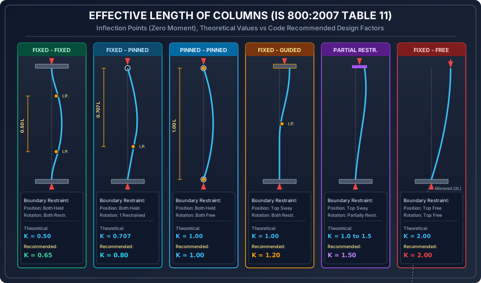
IS 800:2007 Table 11 codifies recommended design values () alongside exact theoretical values () for idealized boundary conditions. The code explicitly mandates using to account for imperfect rotational fixity, bolt slip, and base plate flexibility encountered in real fabrication.
| Case | Boundary Restraint Condition at Ends | Theoretical Value () | Recommended Design Value () | Visual Mode Shape |
|---|---|---|---|---|
| 1 | Effectively held in position and restrained against rotation at both ends (Fixed - Fixed) | Double curvature, two inflection points at | ||
| 2 | Effectively held in position at both ends, restrained against rotation at one end only (Fixed - Pinned) | Inflection point at from fixed base | ||
| 3 | Effectively held in position at both ends, but not restrained against rotation (Pinned - Pinned) | Single half-sine wave, zero inflection points | ||
| 4 | Effectively held in position and restrained against rotation at one end, and at other end restrained against rotation but not held in position (Fixed - Guided Sway) | S-shape sway displacement, inflection point at mid-height | ||
| 5 | Effectively held in position and restrained against rotation at one end, and at other end partially restrained against rotation and not held in position | — | Semi-rigid sway frame column | |
| 6 | Effectively held in position and restrained against rotation at one end, but not held in position nor restrained against rotation at other end (Cantilever / Fixed - Free) | Quarter-sine wave, zero inflection points |
[!IMPORTANT] Theoretical vs Design Multiplier: In competitive examinations, always differentiate between theoretical ( and ) and design ( and ) values. IS 800 adopts and because infinite joint stiffness () is physically unattainable in structural engineering. Base plates and footing connections rotate slightly under high moments.
3. PHYSICAL MECHANICS & FUNDAMENTAL THEORY
3.1 Concept of the Inflection Point (Zero-Moment Node)
In elastic stability theory, when a column deflects under compressive load , the internal bending moment at any section is:
At points where the curvature changes sign (), the internal bending moment is identically zero ().
- These zero-moment points are Points of Contraflexure (Inflection Points).
- Any segment between two inflection points behaves dynamically and statically exactly like a pin-ended Euler strut!
- Consequently, effective length is physically the distance between consecutive points of inflection in the buckled mode shape of the member.
3.2 Cantilever Phenomenon ()
For a column fixed at the base and completely free at the top:
- No point of contraflexure exists within the physical length .
- The column deforms as a quarter-wave of a sine curve.
- By reflecting the buckled shape symmetrically across the fixed base to establish a virtual inflection point, the equivalent full half-wave has a total wavelength of .
- Thus, , causing the elastic Euler buckling capacity to plummet to of the pin-ended value ().
4. MATHEMATICAL DERIVATION & EXACT FORMULATIONS
4.1 Derivation of Euler Critical Load for Classical Boundary Restraints
Case I: Fixed-Fixed Column ()
The general differential equation for column deflection with axial load is:
The general solution is:
Enforcing boundary conditions:
- .
- .
- .
- .
For non-trivial solutions (), the determinant of the coefficient matrix must vanish:
The lowest non-zero buckling mode root gives:
Substituting :
Comparing with standard pin-ended Euler formula :
Case II: Fixed-Pinned Column ()
Enforcing moment equilibrium with lateral reaction :
Solving gives the characteristic transcendental frequency equation:
The smallest positive root occurs at:
4.2 Building Frame Columns: Annex D Restraint Formulation
In multi-story framed buildings, columns are neither isolated nor connected to infinitely rigid supports; they interact elastically with framing beams and adjacent upper/lower column shafts.
Joint Relative Restraint Factor (Clause D.1.2)
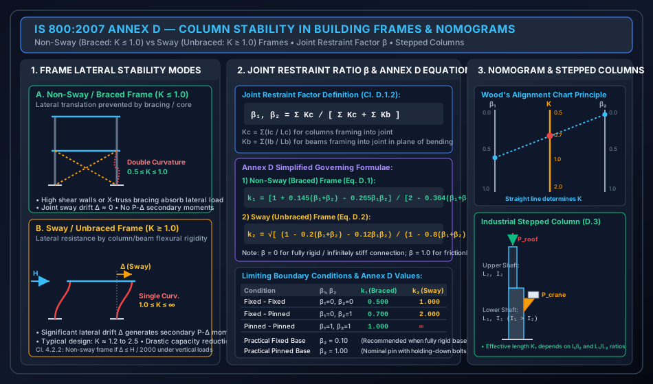
At joint ( at top, at bottom), the rotational restraint factor is given by:
Where:
- is the sum of flexural stiffnesses () of the column shafts framing into joint in the plane of bending.
- is the sum of flexural stiffnesses () of the beams framing into joint in the plane of bending.
- When beams have distant ends fixed or pinned, their effective flexural stiffness is modified:
- Distant end pinned: .
- Distant end fixed: .
Limiting Values of :
- : Beams are infinitely stiff () relative to columns Joint is completely rigid / fully fixed against rotation.
- : Beams have zero stiffness () or connection is pinned Joint is pinned / zero rotational restraint.
- Practical values for foundations:
- Rigid, monolithic base slab on rock or unyielding soil: .
- Nominally pinned base plate with anchor bolts: .
4.3 Governing Equations for Frame Columns (IS 800:2007 Annex D)
1) Non-Sway / Braced Frame (Clause D.1.1, Eq. D.1):
In braced frames (lateral drift prevented by cross-bracing, concrete core walls, or masonry infill panels), :
Verification of boundary limits:
- Fixed-Fixed (): .
- Fixed-Pinned (): .
- Pinned-Pinned (): .
2) Sway / Unbraced Frame (Clause D.1.1, Eq. D.2):
In unbraced frames (lateral loads resisted solely by frame flexural rigidity), lateral drift occurs, :
Verification of boundary limits:
- Fixed-Fixed (): .
- Fixed-Pinned (): .
- Pinned-Pinned (): (Mechanism / instable structure!).
5. STRUCTURAL DETAILING, RESTRAINTS & ALIGNMENT CHARTS
================================================================================
           WOOD'S ALIGNMENT CHART (NOMOGRAM) ARCHITECTURE (ANNEX D)
================================================================================
    Top Joint Factor β₁          Effective Length Factor K       Bottom Joint Factor β₂
          0.0 ────────────────────────────────────────────────────────── 0.0
           │  \                                                        /  │
           │    \                                                    /    │
          0.2     \                                                /     0.2
           │        \                                            /        │
          0.4         \                ● K = 0.61              /         0.4
           │            \            (Braced Frame)          /            │
          0.6 ───────────●─────────────────────────────────●             0.6
           │   (β₁ = 0.597) \                            /  (β₂ = 0.0)    │
          0.8                 \                        /                 0.8
           │                    \                    /                    │
          1.0 ───────────────────\──────────────────/─────────────────── 1.0
================================================================================
5.1 Wood's Alignment Charts
IS 800:2007 provides two nomograms (Fig. 15 for non-sway and Fig. 16 for sway frames).
- Scale on the left vertical axis.
- Scale on the right vertical axis.
- Draw a straight line connecting and .
- The intersection with the central scale gives the effective length factor directly.
5.2 Stepped Columns in Industrial Mill Buildings (Clause D.3)
Heavy industrial buildings with overhead traveling (EOT) cranes utilize stepped columns:
- Lower Shaft (): Heavy built-up or rolled section resisting high vertical crane loads () plus building weight.
- Upper Shaft (): Lighter section carrying roof truss reactions () only ().
- The effective length factor of the lower shaft is obtained from Annex D.3 charts based on:
- Slenderness of the lower shaft is computed as:
6. HIGH-IMPACT VISUAL ARCHITECTURE
6.1 Classical End Restraints & Effective Length Multipliers
The diagram below illustrates the 6 classical IS 800:2007 Table 11 boundary configurations, their theoretical vs recommended design factors, and buckled mode shapes showing inflection point positions.
6.2 Multi-Story Frame Stability & Annex D Nomograms
The diagram below illustrates the fundamental behavioral difference between braced (non-sway) and unbraced (sway) building frames, joint restraint factor formulations, and industrial stepped column mechanics.
7. CODE NUANCES, EXCEPTIONS & DESIGN GUARDRAILS
7.1 Sway Classification Criterion (Clause 4.2.2)
A building frame is categorized as Non-Sway if:
- Under nominal vertical loads, the lateral sway displacement in any story satisfies: Where is the story height.
- Alternatively, if the total lateral bracing system (shear wall or diagonal bracing) provides at least of the total lateral stiffness of the structure.
7.2 Weak-Axis Column Bracing in Industrial Sheds
- In steel shed portal frames, columns are framed rigidly about their major axis (-) to form a moment-resisting bent ().
- Along the longitudinal axis (-), girts, side runners, and longitudinal tie-bracings are placed at intermediate heights (e.g., at or ).
- Therefore:
- Always check both axes! A column may fail about its major axis if weak-axis intermediate ties reduce significantly!
8. STANDARD WORKED NUMERICAL EXAMPLES
================================================================================
             VERIFIED NUMERICAL CALCULATION SUMMARY (IS 800:2007)
================================================================================
  Example 1: Multi-Story Column (ISHB 300, L = 4.0 m, β₁ = 0.5966, β₂ = 0.0)
    • Non-Sway (Braced): k₁ = 0.6094  => KL = 2437.6 mm => λ = 18.82 => Pd = 1700.9 kN
    • Sway (Unbraced):   k₂ = 1.2980  => KL = 5192.0 mm => λ = 40.09 => Pd = 1539.7 kN
    • Sway Penalty: Effective length increased by 113.0%, reducing load capacity by 161.2 kN.

  Example 2: Classical Table 11 Boundary Comparison (ISHB 250, L = 4.5 m, Curve c)
    • Fixed - Fixed (K_des = 0.65):   KL = 2925 mm, λ = 53.28, f_cd = 178.59 MPa, Pd = 1245.0 kN
    • Fixed - Pinned (K_des = 0.80):  KL = 3600 mm, λ = 65.57, f_cd = 159.45 MPa, Pd = 1111.5 kN
    • Pinned - Pinned (K_des = 1.00): KL = 4500 mm, λ = 81.97, f_cd = 133.20 MPa, Pd = 928.5 kN
    • Cantilever (K_des = 2.00):      KL = 9000 mm, λ = 163.93, f_cd = 51.14 MPa,  Pd = 356.5 kN
    • Capacity Gain: Fixed-Fixed column carries +249.2% higher axial load than Cantilever!

  Example 3: Stepped Crane Column (Annex D.3, L₁ = 6.0 m, I₁/I₂ = 5.0, L₁/L₂ = 2.0)
    • Effective Length Factor: K₁ = 1.65 => KL₁ = 9900 mm => λ₁ = 46.22
    • Fe 410 Steel (Curve b): f_cd = 198.93 MPa => Pd₁ = 3680.2 kN >= P_tot = 850.0 kN (SAFE)
================================================================================
8.1 Example 1: Multi-Story Frame Column — Sway vs Non-Sway (IS 800 Annex D)
Problem Statement:
An interior ground-floor column of a multi-story office building has an unsupported length . The column is an ISHB 300 @ 58.8 kg/m (, , , , , ).
- At Top Joint A: The column connects to an upper column (, same ISHB 300) and two identical framing beams (ISMB 350, span , ).
- At Bottom Joint B: The column is rigidly fixed into a heavy reinforced concrete pile cap footing ().
Calculate the effective length factor and design compressive strength about the major axis (-) if the frame is:
- Braced against lateral sway (Non-sway frame).
- Unbraced against lateral sway (Sway frame).
Steel grade Fe 410 (, , ).
Step-by-Step Mathematical Solution:
Step 1: Member Flexural Stiffness Calculations
At Joint A:
- Lower column stiffness:
- Upper column stiffness:
- Total column stiffness at joint:
- Framing beam stiffness (two beams frame into joint in plane of bending):
Step 2: Joint Restraint Factor and
At foundation base (ideal monolithic fixed support):
Step 3: Effective Length Factor for Non-Sway (Braced) Frame
Using IS 800:2007 Annex D Eq. D.1:
Slenderness ratio about major axis:
Euler critical stress:
Non-dimensional slenderness:
For ISHB 300 major axis buckling (, ), Table 10 prescribes Curve b ():
Step 4: Effective Length Factor for Sway (Unbraced) Frame
Using IS 800:2007 Annex D Eq. D.2:
Slenderness ratio:
Euler critical stress:
Non-dimensional slenderness:
Design stress parameter (Curve b, ):
Stress reduction factor :
Physical Insight: Allowing lateral sway doubles the effective column length (), reducing the column capacity by ( reduction in short-column regime, escalating to in slender columns).
8.2 Example 2: Comparative Study of IS 800 Table 11 Boundary Conditions
Problem Statement:
An ISHB 250 @ 54.7 kg/m column has an actual unsupported height .
Properties: , , , , .
Steel grade Fe 410 (, , ). Minor axis buckling governs ( Table 10 Curve c, ).
Compute and compare the design compressive strength for:
- Both ends fixed ().
- One end fixed, other pinned ().
- Both ends pinned ().
- Cantilever / Fixed at base, free at top ().
Step-by-Step Computational Results:
Case 1: Fixed-Fixed ()
Case 2: Fixed-Pinned ()
Case 3: Pinned-Pinned ()
Case 4: Cantilever ()
Synthesis:
8.3 Example 3: Industrial Stepped Crane Column (IS 800 Annex D.3)
Problem Statement:
A heavy industrial workshop mill bent has a stepped column.
- Lower shaft (): Carries gantry crane bracket. , , .
- Upper shaft (): Carries roof truss. , , .
- Loads: Crane vertical wheel load at seat , roof truss vertical reaction at top . Total axial load on lower shaft .
- Column base is rigidly fixed, and top is guided by the roof bent. From Annex D.3 charts for , , and , the lower shaft effective length factor is . Check the structural safety of the lower column shaft using Fe 410 steel (Curve b, , , ).
Step-by-Step Mathematical Solution:
- Effective length of lower shaft:
- Slenderness ratio:
- Euler critical stress:
- Non-dimensional slenderness:
- Design compressive stress (Table 7, Curve b, ):
- Design Compressive Strength:
- Safety Check:
9. COMPARATIVE ANALYSIS & DESIGN OPTIMIZATION
| Parameter | Theoretical Euler Mechanics | IS 800:2007 Table 11 Recommendations | IS 800 Annex D Frame Analysis |
|---|---|---|---|
| Joint Modeling | Pure mathematical points (100% rigid or frictionless pin) | Realistic semi-rigid connection allowances () | Exact joint stiffness ratio |
| Fixed-Fixed Column | (+30% length penalty for base flexibility) | only if | |
| Fixed-Pinned Column | (+13% length penalty) | when | |
| Sway Behavior | Uncoupled bifurcation analysis | Empirical multipliers | Explicit differentiation between Non-Sway () and Sway () |
| Application Scope | Academic textbook derivations | Individual isolated columns, preliminary sizing | High-rise multistory buildings, portal frames, industrial bents |
10. COMMON PITFALLS, SITE ERRORS & EXAMINATION TRAPS
10.1 Pitfall 1: Confusing Theoretical () and Design () Values
- In competitive examinations (GATE & ESE), question setters often frame: "As per IS 800:2007, the effective length of a column effectively held in position and restrained against rotation at both ends is..."
- If the options contain both and , is the correct answer as per Table 11! Only choose if the question explicitly specifies "theoretically" or "Euler ideal boundary".
10.2 Pitfall 2: Neglecting Sway Status in Portal Frames
- Engineers often assume for columns in single-story portal frames pinned at the base.
- Fatal Error: If the roof diaphragm or portal ridge is not braced against lateral sidesway, the frame will sway under gravity and wind loads!
- For a portal column pinned at base and rigid at eaves without sway bracing:
- Assuming instead of overestimates column capacity by up to , leading to progressive collapse!
10.3 Pitfall 3: Intermediate Purlin/Girt Bracing Axis Confusion
- Cladding girts attached to the outer flange of a column brace the column against minor-axis buckling (-) only.
- They do not brace the column against major-axis buckling (-) in the plane of the frame.
- Always calculate: Where is the girt spacing (typically or ). The governing slenderness is .
11. MULTI-EXAM PREPARATION MATRIX
| Exam Pattern | High-Yield Topics & Question Formats | Key Formulas & Memory Aids |
|---|---|---|
| GATE CE | • Exact computation of Annex D from joint stiffnesses • Transcendental stability equations • Biaxially braced column slenderness checking () |
check |
| UPSC ESE | • Direct memory retrieval of Table 11 vs (all 6 cases) • Sway drift limit (Cl. 4.2.2) • Stepped crane column mechanics and Annex D.3 charts |
Fixed-Fixed: Fixed-Pinned: Cantilever: Fixed-Guided: |
| SSC JE / RRB JE | • Direct one-liner questions on Table 11 effective length factors • Distance between inflection points definition • Slenderness ratio calculation for cantilever struts |
Cantilever: Pinned ends: |
| State AE / JE | • Comparison between non-sway () and sway () columns • Boundary factor (rigid) vs (pin) • Numerical problems on calculation |
Rigid base: Hinged base: |
12. COMPREHENSIVE REFERENCES & CROSS-LINKING
- Upstream Theory: 01_column_buckling_theory_and_curves.md — Euler buckling theory, Perry-Robertson formulation, and IS 800:2007 buckling curves a, b, c, d.
- Downstream Module: 03_built_up_columns_lacing_battening.md — Built-up compression members, lacing systems (Cl. 7.6), and battened columns (Cl. 7.7).
- Primary Standards:
- Bureau of Indian Standards, IS 800:2007, General Construction in Steel — Code of Practice, Section 7 and Annex D.
- S. K. Duggal, Limit State Design of Steel Structures, McGraw Hill India, 3rd Edition.
- N. Subramanian, Design of Steel Structures, Oxford University Press.