Column Buckling Theory & Perry-Robertson Formulation (IS 800:2007 Cl. 7.1)
In this chapter (4 topics)
On this page
- 1. Engineering Context & Overview
- The Bifurcation & Real Column Dilemma
- 2. Classical Euler Column Buckling Theory & Assumptions
- 2.1 Euler Buckling Load Derivation
- 2.2 Euler Critical Buckling Stress (fcr)
- 2.3 Limitations & Failure of Euler Theory for Real Columns
- 3. Real Column Mechanics & The Perry-Robertson Formulation
- 3.1 Initial Crookedness & Deflection Amplification
- 3.2 Cross-Sectional Stress Superposition
- 3.3 The Perry-Robertson Quadratic Equation
- 4. Governing Indian Standard Code Provisions (IS 800:2007 Cl. 7.1.2)
- 4.1 Design Compressive Stress Formulation (fcd)
- 4.2 Parameter Definitions & The Plastic Plateau
- 4.3 Design Compressive Strength (Pd)
- 5. Multiple Column Buckling Curves (a, b, c, d) and Selection Matrix
- 5.1 Physical Basis of the Four Curves
- 5.2 Table 7 Imperfection Factors (α)
- 5.3 IS 800:2007 Table 10 Selection Matrix
- 6. Cross-Section Classification per IS 800:2007 Table 2
- 6.1 The Four Behavioral Classes
- 7. Architectural SVG Technical Illustrations
- 7.1 Column Buckling Curves and Imperfection Mechanics
- 7.2 Perry-Robertson Stress State and Cross-Section Classes
- 8. Step-by-Step Pre-Calculated Numerical Problems
- Problem 1: Compressive Load Capacity of Rolled Steel Column (ISMB 400)
- Problem 2: Comparative Analysis of All 4 Buckling Curves (a, b, c, d)
- Problem 3: Square Hollow Section (SHS) Hot-Finished vs Cold-Formed
- 9. Comprehensive Summary & Comparative Analysis Table
- 10. Critical Practical Design & Detailing Guidelines
- 11. Site Pitfalls, Fabrication Blunders & Inspection Failures
- 12. Competitive Examination Traps & Multiple-Choice Practice Questions
- Trap 1: The Plastic Plateau Slenderness Limit
- Trap 2: Major vs Minor Axis Buckling Curves
- Trap 3: Imperfection Factor Order
- Practice Question 1 (GATE CE)
- Practice Question 2 (UPSC ESE)
- Practice Question 3 (SSC JE / State AE)
1. Engineering Context & Overview
In structural steel framing—encompassing high-rise buildings, industrial mill workshops, offshore platforms, highway truss bridges, and power transmission towers—compression members are primary load-carrying elements that transfer axial compressive thrusts. Common structural forms include:
- Columns / Stanchions: Heavy vertical members supporting gravity and lateral building loads.
- Struts: Inclined or horizontal compressive web members in roof trusses and open-web joists.
- Boom Members / Chords: Top chord compression elements in simply supported bridge trusses.
- Piers & Tower Legs: Heavily stressed compressive columns in transmission pylons and industrial bents.
Unlike tension members—which fail when axial stress reaches the material yield or ultimate tensile strength—compression members frequently collapse at stresses far below the yield strength () due to a geometric phenomenon known as buckling (loss of lateral stability).
The Bifurcation & Real Column Dilemma
In classical elastic stability theory, an ideal, perfectly straight column undergoes a bifurcation of equilibrium at the Euler critical load (). However, real civil engineering columns never achieve the theoretical Euler capacity in the practical slenderness range (). Real structural columns exhibit unavoidable physical defects:
- Geometric Imperfections: Initial out-of-straightness (crookedness or initial bow ) resulting from hot-rolling, cooling, and handling tolerances.
- Thermal Residual Stresses: Severe internal cooling stresses developed during manufacture (flange tips of rolled I-sections cool rapidly, locking in compressive residual stresses of ).
- Accidental Load Eccentricity: Unavoidable misalignments at bolted column splices and beam-to-column beam seat connections.
To reconcile theory with extensive experimental testing conducted across international laboratories (most notably the European Convention for Constructional Steelwork, ECCS), the modern Indian Standard Code of Practice for General Construction in Steel (IS 800:2007, Clause 7.1.2) abandoned archaic empirical Rankine-Gordon formulas. In their place, IS 800:2007 adopted the Perry-Robertson formulation expressed through four distinct non-dimensional column buckling curves (Curves a, b, c, and d).
2. Classical Euler Column Buckling Theory & Assumptions
2.1 Euler Buckling Load Derivation
Consider an ideal, perfectly straight, pin-ended column of length , cross-sectional area , moment of inertia , and modulus of elasticity . Under an increasing axial load , the column remains perfectly straight until reaches a critical threshold , at which point it can maintain equilibrium in a slightly bent configuration.
       P (Axial Thrust)
       ↓
     ┌───┐ (Pin Support)
     │   │
     │ ( │ <── Lateral Deflection y(x)
     │   │
     └───┘ (Pin Support)
       ↑
       P
Taking the coordinate along the column length from the bottom pin and as the lateral deflection:
- The internal bending moment at any section is:
- From elementary Bernoulli-Euler beam theory:
- Setting , the general solution of this second-order homogeneous differential equation is:
- Applying boundary conditions:
- At , .
- At , .
- For a non-trivial buckled shape (), we must have:
- The fundamental (lowest) buckling mode corresponds to :
- Squaring both sides yields the classical Euler Critical Buckling Load:
where is the effective length accounting for boundary restraint conditions.
2.2 Euler Critical Buckling Stress ()
Expressing the moment of inertia in terms of the radius of gyration (, where ):
Dividing by the cross-sectional area gives the Euler Critical Stress ():
where is the slenderness ratio of the column.
2.3 Limitations & Failure of Euler Theory for Real Columns
Euler's equation is based on ideal assumptions:
- The column is perfectly straight, homogeneous, and isotropic.
- The compressive load is applied perfectly axially along the centroidal axis.
- The material remains linearly elastic throughout buckling ().
Why Euler Theory Overpredicts Capacity:
- For very slender columns (), buckling occurs at stresses well below the proportional limit; Euler theory matches experimental data closely.
- For intermediate columns (), which comprise over of real civil engineering columns, Euler theory drastically overestimates capacity (sometimes by ). In this range, residual stresses and geometric crookedness cause localized yielding long before the theoretical Euler bifurcation point is reached.
3. Real Column Mechanics & The Perry-Robertson Formulation
3.1 Initial Crookedness & Deflection Amplification
Real columns have an initial sinusoidal curvature before any load is applied:
where is the initial amplitude at mid-height (typically ).
When an axial compressive load is applied, the initial deflection induces an eccentric moment . The governing differential equation becomes:
Solving this non-homogeneous equation demonstrates that the lateral deflection amplifies into:
The maximum mid-span deflection is:
where is the average axial compressive stress and .
3.2 Cross-Sectional Stress Superposition
The maximum compressive stress occurs in the extreme concave fiber at mid-span, combining uniform direct axial thrust and amplified flexural bending stress:
Substituting and noting that section modulus (where is the distance from the neutral axis to the extreme fiber):
3.3 The Perry-Robertson Quadratic Equation
Defining the non-dimensional imperfection parameter :
The peak stress becomes:
Perry and Robertson postulated that column failure initiates when the maximum extreme fiber stress reaches the material yield strength :
Multiplying through by :
Multiplying across by yields the classic Perry-Robertson Quadratic Formula:
or in factored form:
Solving this quadratic equation for the compressive stress gives the characteristic compressive resistance of the real column.
4. Governing Indian Standard Code Provisions (IS 800:2007 Cl. 7.1.2)
In IS 800:2007 Clause 7.1.2.1, the Perry-Robertson formulation is normalized into a limit-state design equation by introducing the non-dimensional slenderness ratio () and partial safety factor .
4.1 Design Compressive Stress Formulation ()
The design compressive stress of an axially loaded compression member shall be calculated from:
where:
4.2 Parameter Definitions & The Plastic Plateau
- = Design compressive stress ().
- = Characteristic yield stress of the steel ().
- = Partial safety factor for resistance governed by yielding (Table 5).
- = Non-dimensional effective slenderness ratio.
- = Imperfection factor corresponding to the appropriate buckling curve (Table 7).
- = Auxiliary calculation factor combining slenderness and initial imperfection.
- = Stress reduction factor ().
- The Plastic Plateau ():
For stocky columns with non-dimensional slenderness (equivalent to for Fe 410 steel), geometric imperfections and residual stresses have negligible destabilizing effects. The column yields plastically across its full cross-section without buckling:
4.3 Design Compressive Strength ()
The design compressive strength of a column is:
where is the effective cross-sectional area:
- For Class 1 (Plastic), Class 2 (Compact), and Class 3 (Semi-Compact) sections: (gross cross-sectional area).
- For Class 4 (Slender) sections: is the reduced effective area accounting for local plate buckling per Clause 7.3.2.
5. Multiple Column Buckling Curves (a, b, c, d) and Selection Matrix
5.1 Physical Basis of the Four Curves
Why does IS 800 provide four distinct curves rather than a single formula?
Because structural shapes possess wildly divergent residual stress magnitudes and cross-sectional geometries:
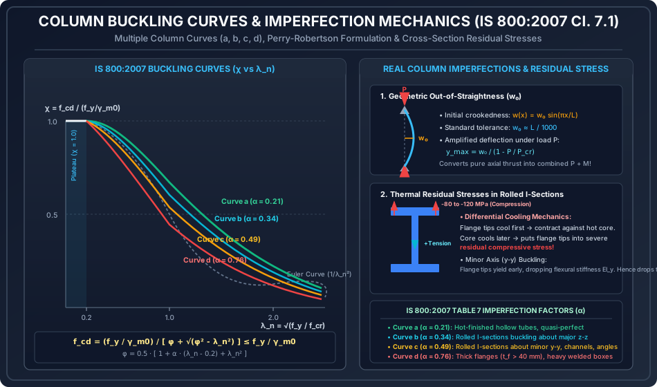
- Curve a (): Represents sections with minimal residual stresses and quasi-perfect geometries (e.g., hot-finished seamless hollow sections, stress-relieved rolled shapes). Exhibits highest load-carrying efficiency.
- Curve b (): Represents rolled I-sections buckling about their major axis () and welded box sections. Flange tips undergo moderate residual compression, but major axis flexural inertia () mitigates premature instability.
- Curve c (): Represents rolled I-sections buckling about their minor axis (), channel sections, structural angles, T-sections, and cold-formed hollow tubes. Flange tip residual compression heavily degrades minor axis inertia (), causing substantial capacity reduction.
- Curve d (): Represents heavy rolled sections with very thick flanges (), thick-welded box girders, and heavy solid steel billets. High thermal mass creates massive residual tensile cores and deep compressive zones, causing severe early yielding.
5.2 Table 7 Imperfection Factors ()
| Buckling Curve | Imperfection Factor () | Representative Structural Sections |
|---|---|---|
| a | Hot-finished hollow circular/square sections, quasi-perfect rolled bars. | |
| b | Rolled I-sections () buckling about major axis ; welded box sections. | |
| c | Rolled I-sections buckling about minor axis ; channels, angles, tees, cold-formed tubes. | |
| d | Heavy rolled I-sections with ; thick welded sections; solid round shafts. |
5.3 IS 800:2007 Table 10 Selection Matrix
| Cross-Section Category | Dimensional Limits | Buckling About Axis | Buckling Curve |
|---|---|---|---|
| Rolled I-Sections | and | (Major) (Minor) |
Curve a Curve b |
| and | (Major) (Minor) |
Curve b Curve c |
|
| (Major) (Minor) |
Curve c Curve d |
||
| Welded I-Sections | (Major) (Minor) |
Curve b Curve c |
|
| (Major) (Minor) |
Curve c Curve d |
||
| Hollow Sections | Hot-Finished (Seamless/Welded) Cold-Formed |
Any Axis Any Axis |
Curve a Curve c |
| Channels, Angles, Tees | Any standard rolling | Any Axis | Curve c |
| Built-up Laced/Battened | Any structural configuration | Any Axis | Curve c (Cl. 7.6.1.5) |
6. Cross-Section Classification per IS 800:2007 Table 2
To prevent localized plate buckling from precipitating global member collapse before the calculated is mobilized, cross-sections must be classified according to their component width-to-thickness ratios (, , ).
            b = b_f / 2 (Outstand)
           ├─────────┤
          ┌───────────┐ ┬
          │           │ │ t_f
          └─────┬─────┘ ┴
                │
                │ Web depth d
                │ t_w
                │
          ┌─────┴─────┐
          │           │
          └───────────┘
The yield stress ratio parameter is defined as:
6.1 The Four Behavioral Classes
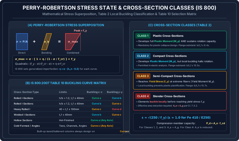
- Class 1 (Plastic): Cross-sections capable of developing a fully plastic hinge moment () and sustaining the rotation capacity () required for plastic collapse analysis without local buckling.
- Flange outstand:
- Web under neutral axis at mid-depth:
- Class 2 (Compact): Cross-sections that can develop the plastic moment capacity (), but localized buckling halts further plastic rotation capacity. Permitted for elastic global analysis.
- Flange outstand:
- Web under neutral axis at mid-depth:
- Class 3 (Semi-Compact): Cross-sections where the extreme fiber stress can reach yield strength (), developing the elastic yield moment (), but localized buckling prevents advancement to full plastic moment.
- Flange outstand:
- Web under neutral axis at mid-depth:
- Class 4 (Slender): Cross-sections where component plates buckle locally before yield stress is reached.
- Flange outstand:
- In compression members, Class 4 sections suffer from premature localized wrinkling; the member must be designed using an effective reduced area () per Clause 7.3.2.
7. Architectural SVG Technical Illustrations
7.1 Column Buckling Curves and Imperfection Mechanics
The following diagram illustrates the four European/IS 800 buckling curves (a, b, c, d) plotted as non-dimensional design stress versus , along with physical depictions of initial out-of-straightness () and cross-sectional residual stresses in rolled I-sections.
7.2 Perry-Robertson Stress State and Cross-Section Classes
This diagram details the stress superposition principle of the Perry-Robertson formulation, the Table 10 selection matrix, and the four cross-section behavioral classes of IS 800 Table 2.
8. Step-by-Step Pre-Calculated Numerical Problems
Problem 1: Compressive Load Capacity of Rolled Steel Column (ISMB 400)
A rolled steel beam section ISMB 400 is used as an axially loaded column of unsupported length with both ends pinned ().
- Steel grade: Fe 410 ().
- Section properties from steel tables:
- Gross area
- Overall depth , Flange width
- Flange thickness , Web thickness
- Radii of gyration: ,
Determine:
- Cross-section classification per IS 800:2007 Table 2.
- Governing slenderness ratio and applicable buckling curve per Table 10.
- Design compressive stress per IS 800:2007 Cl. 7.1.2.
- Factored axial compressive load capacity .
Solution & Step-by-Step Calculations:
Step 1: Check Cross-Section Classification (IS 800:2007 Table 2)
- Yield parameter:
- Flange outstand:
Table 2 limit for Class 1 (Plastic): .
Since , the flange is Class 1 (Plastic). - Web clear depth:
Table 2 limit for Class 1 (neutral axis at mid-depth): .
Since , the web is Class 1 (Plastic). - Section Classification: The overall cross-section is Class 1 (Plastic/Compact).
Therefore, no local buckling reduction is required:
Step 2: Determine Governing Slenderness Ratio & Buckling Curve
- Effective length: .
- Slenderness about major axis ():
- Slenderness about minor axis ():
- Governing slenderness ratio:
Step 3: Select Buckling Curve from Table 10
- Section aspect ratio:
- Flange thickness .
- From IS 800 Table 10:
- For and , buckling about minor axis corresponds to Buckling Curve c.
- From Table 7: Imperfection factor for Curve c is .
Step 4: Compute Design Compressive Stress ()
- Euler critical buckling stress:
- Non-dimensional effective slenderness:
- Auxiliary factor :
- Stress reduction factor :
- Design compressive stress:
Step 5: Compute Factored Compressive Load Capacity ()
Problem 2: Comparative Analysis of All 4 Buckling Curves (a, b, c, d)
For a structural steel column with slenderness ratio , steel grade Fe 410 (), quantify the impact of initial imperfections and residual stresses by calculating for each of the four buckling curves.
Solution & Step-by-Step Calculations:
Step 1: Common Baseline Elastic Properties
- Yield design stress:
- Euler critical buckling stress:
- Non-dimensional slenderness: Notice that and .
Step 2: Calculate for Curve a (, Hot-finished tubes)
Step 3: Calculate for Curve b (, Rolled I-sections z-z)
Step 4: Calculate for Curve c (, Rolled I-sections y-y, angles)
Step 5: Calculate for Curve d (, Thick flanges )
Summary Comparison Table ():
| Buckling Curve | Reduction Factor | (MPa) | Reduction from Plastic Yield () | ||
|---|---|---|---|---|---|
| Curve a | |||||
| Curve b | |||||
| Curve c | |||||
| Curve d |
Key Structural Insight: For the identical slenderness (), shifting from Curve a (hot-finished tube) to Curve d (thick-welded section) drops the allowable compressive stress from to —a loss in allowable stress solely due to cross-sectional residual stress and geometric imperfection severity!
Problem 3: Square Hollow Section (SHS) Hot-Finished vs Cold-Formed
A square structural column uses an SHS section () over an effective length .
- Determine the design compressive strength if the section is Hot-Finished (Curve a, ).
- Determine if the section is Cold-Formed (Curve c, ).
- Calculate the percentage strength advantage provided by the hot-finished manufacturing process.
Solution & Step-by-Step Calculations:
Step 1: Compute Slenderness Ratio & Baseline Stress
- Euler stress:
- Non-dimensional slenderness:
Step 2: Hot-Finished Section (Curve a, )
- Auxiliary factor:
- Reduction factor:
- Compressive stress and capacity:
Step 3: Cold-Formed Section (Curve c, )
- Auxiliary factor:
- Reduction factor:
- Compressive stress and capacity:
Step 4: Strength Advantage Evaluation
Design Takeaway: Specifying a hot-finished structural tube yields nearly a increase in axial compressive load capacity over an identical cold-formed tube, providing substantial steel weight savings in high-load industrial structures.
9. Comprehensive Summary & Comparative Analysis Table
| Characteristic / Parameter | Euler Classical Theory | Rankine-Gordon Formula (Old IS 800:1984) | Perry-Robertson Modern Code (IS 800:2007) |
|---|---|---|---|
| Physical Formulation | Pure bifurcation of perfect elastic column. | Semi-empirical interaction: . | Mathematical stress superposition with initial bow () and residual stress. |
| Material Behavior | Infinite linear elasticity assumed. | Transition between yield and elastic buckling. | Explicit yield envelope with multiple imperfection factors (). |
| Account of Imperfections | Completely ignored (). | Approximated via single empirical constant . | Explicitly modeled through 4 curves (a, b, c, d) matching ECCS experimental databases. |
| Accuracy in Practical Range () | Highly unconservative (overpredicts by up to ). | Coarse approximation; fails to capture residual stress nuances. | Excellent correlation with full-scale column tests worldwide. |
| Safety Factors Applied | Factor of Safety required. | Working Stress Method (Factor of Safety ). | Limit State Method: Partial safety factor . |
10. Critical Practical Design & Detailing Guidelines
- Orientation of Rolled I-Sections:
In standard rolled beams (ISMB, ISLB), the major radius of gyration is dramatically higher than the minor radius (). Under equal unsupported lengths (), buckling about the minor axis always governs, resulting in severe capacity drops (Curve c). To maximize economy:
- Provide intermediate lateral bracings in the weak direction to reduce .
- For unbraced columns, select wide-flange column sections (ISSC, ISHB) or square hollow sections where .
- Preventing Local Buckling: Always verify Table 2 width-to-thickness limits before computing . If a section is Class 4 (Slender), the engineer cannot use the gross area ; the reduced effective area must be calculated per Cl. 7.3.2, or plate stiffeners added.
- Flange Thickness Transition Threshold (): When designing heavy transfer columns in multi-story buildings, note that when flange thickness exceeds (), the section shifts down by one full buckling curve (e.g., from Curve b to Curve c, or from Curve c to Curve d), substantially reducing design stress.
11. Site Pitfalls, Fabrication Blunders & Inspection Failures
- Straightening Damaged Columns with Direct Flame: When rolled columns bent during transit are flame-straightened on site without controlled preheating, severe uncalculated residual stresses are introduced. This can drop a member's buckling performance from Curve b down below Curve d, leading to unexpected buckling under service loads.
- Substituting Cold-Formed Tubes for Hot-Finished Tubes: Fabricators frequently substitute cheaper cold-formed hollow sections for specified hot-finished tubes without redesigning for Curve c () instead of Curve a (). As demonstrated in Problem 3, this results in an immediate deficit in compressive capacity.
- Ignoring Weak-Axis Restraint Inadequacy: Designers assume pinned weak-axis restraint from masonry infill or light cladding rails. If the connection cannot resist the mandatory stabilizing force required by Cl. 7.5.2, the column will buckle over its full unsupported height.
12. Competitive Examination Traps & Multiple-Choice Practice Questions
Trap 1: The Plastic Plateau Slenderness Limit
Trap: In competitive exams, candidates often believe that no reduction in compressive stress occurs up to or . Fact: The plastic plateau in IS 800:2007 Cl. 7.1.2.1 extends strictly up to . For Fe 410 steel (), this corresponds to an actual slenderness of only ! Above , stress reduction begins immediately.
Trap 2: Major vs Minor Axis Buckling Curves
Trap: Assuming an ISMB column uses Curve a for all buckling modes. Fact: For rolled I-sections with , major axis buckling () uses Curve a, but minor axis buckling () uses Curve b! For , major axis uses Curve b and minor axis uses Curve c!
Trap 3: Imperfection Factor Order
Trap: Confusing the numerical values of for curves a, b, c, d. Mnemonic: Remember (Roughly increasing by ).
Practice Question 1 (GATE CE)
Q: In IS 800:2007, the design compressive stress of an axially loaded compression member is based on the Perry-Robertson formulation. The non-dimensional slenderness ratio up to which the design compressive stress is taken as without any buckling reduction (the plastic plateau) is:
- (A)
- (B)
- (C)
- (D)
Answer: (B)
Explanation: Per IS 800:2007 Clause 7.1.2.1, for , the reduction factor , and .
Practice Question 2 (UPSC ESE)
Q: A hot-rolled steel I-section with overall depth and flange width has a flange thickness . If the column buckles about its minor axis (), which buckling curve per IS 800:2007 Table 10 shall be adopted?
- (A) Curve a
- (B) Curve b
- (C) Curve c
- (D) Curve d
Answer: (B)
Explanation:
- Ratio .
- Flange thickness .
- Per IS 800:2007 Table 10, for rolled I-sections with and , buckling about the major axis corresponds to Curve a, while buckling about the minor axis corresponds to Curve b (whereas if and , is Curve b and is Curve c). Since , minor axis buckling uses Curve b!
Practice Question 3 (SSC JE / State AE)
Q: As per IS 800:2007 Table 7, what is the value of the imperfection factor for Buckling Curve c?
- (A)
- (B)
- (C)
- (D)
Answer: (C)
Explanation: The imperfection factors defined in Table 7 are:
- Curve a:
- Curve b:
- Curve c:
- Curve d:
Therefore, Option (C) is correct.