Subsurface Exploration & Soil Investigation
In this chapter (5 topics)
On this page
- 1. Module Overview & Learning Objectives
- Primary Learning Objectives:
- 2. Scope & Objectives of Subsurface Exploration
- Depth of Exploration (Dexp):
- 3. Methods of Exploration & Boring (IS 1892:1979)
- Rock Coring Parameters (IS 11315):
- 4. Soil Sampling & Sampler Geometrical Design Criteria
- Sampler Design Geometrical Parameters (IS 1892 / IS 2132):
- 1. Area Ratio (Ar):
- 2. Inside Clearance Ratio (Ci):
- 3. Outside Clearance Ratio (Co):
- 4. Recovery Ratio (Lr):
- 5. Standard Penetration Test (SPT - IS 2131:1981)
- Standard Test Specifications (IS 2131):
- Test Execution Procedure:
- 6. Dual Corrections to Observed SPT N-Value
- Step 1: Overburden Pressure Correction (N1):
- Step 2: Dilatancy (Water Table) Correction (Ncorrected):
- 7. Cone Penetration Testing (CPT & CPTu Piezocone)
- Mechanical & Electric Cone Specifications:
- Measured CPT Parameters:
- Soil Behavior Type (SBT) Classification:
- Piezocone (CPTu) & Pore Pressure Transducer (u2):
- 8. Geophysical Exploration: Seismic Refraction Method
- Fundamental Physical Principle (Snell's Law):
- Time-Distance Relationship & Formulations:
- Depth to Bedrock (H1):
- The "Hidden Layer" / Blind Zone Limitation:
- 9. Electrical Resistivity Methods (Wenner & Schlumberger)
- Wenner Electrode Configuration:
- Profiling vs. Sounding:
- 10. Subsoil Investigation Report (IS 1892)
- 11. Solved Numerical Problems
- Problem 1: Soil Sampler Geometry & Core Recovery Evaluation
- Problem 2: Standard Penetration Test Multi-Level Corrections
- Problem 3: Seismic Refraction Subsurface Layer Thickness Determination
- 12. Comparative Engineering Analysis Across Syllabi
- 13. Common Misconceptions & Examination Pitfalls
- 14. Key Reference Formulas & Summary Table
1. Module Overview & Learning Objectives
Geotechnical site exploration forms the absolute empirical foundation upon which all structural foundation designs, slope stability evaluations, and earth-retaining structures depend. Inadequate or erroneous subsurface characterization is the single largest contributing factor to catastrophic foundation failures, excessive differential settlements, and construction litigation.
                           SUBSURFACE EXPLORATION METHODS
                                         │
              ┌──────────────────────────┴──────────────────────────┐
              ▼                                                     ▼
      DIRECT METHODS (BORING & SAMPLING)                  IN-SITU FIELD & GEOPHYSICAL
              │                                                     │
    ┌─────────┴─────────┐                                 ┌─────────┴─────────┐
    ▼                   ▼                                 ▼                   ▼
 Boring Methods     Soil Sampling                      Penetration Tests   Geophysical Surveys
 (Trial Pits,       (Disturbed vs. UDS,                (SPT, CPT, CPTu,    (Seismic Refraction,
  Auger, Wash,       Area Ratio A_r,                    Dilatancy &         Electrical Resistivity
  Rotary Coring)     Clearance Ratios C_i, C_o)         Overburden Corr.)   Wenner/Schlumberger)
Primary Learning Objectives:
- Master Boring & Drilling Techniques: Evaluate the operational mechanics, advantages, and limitations of trial pits, auger boring, wash boring, percussion drilling, and rotary diamond coring.
- Formulate Sampler Disturbance Criteria: Derive and apply the mathematical design formulations for Area Ratio (), Inside Clearance (), Outside Clearance (), and Recovery Ratio () under IS 1892 / IS 2132.
- Execute Standard Penetration Testing (SPT): Apply the standardized IS 2131 procedure ( hammer, fall, three drives) and enforce the strict sequence of Overburden Correction followed by Dilatancy Correction.
- Interpret Cone Penetration Tests (CPT/CPTu): Classify subsoils into Soil Behavior Types (SBT) using cone resistance (), sleeve friction (), and friction ratio ().
- Analyze Geophysical Wave Refraction: Apply Snell's Law to calculate the critical angle , bedrock depth , and cross-over distance from time-distance seismograms, identifying blind-zone limitations.
- Formulate Electrical Resistivity Surveys: Compute apparent resistivity under Wenner and Schlumberger electrode arrays.
2. Scope & Objectives of Subsurface Exploration
Under IS 1892:1979, the scope of a geotechnical exploration program is tailored to establish:
- The vertical sequence, thickness, dip, and lateral extent of distinct soil and rock strata.
- The elevation of the groundwater table, its seasonal fluctuations, and the presence of artesian pore water pressures.
- Engineering properties of the subsoil: shear strength parameters (), compressibility (), permeability (), and compaction characteristics.
- Chemical agressiveness of groundwater and subsoil (sulfate and chloride content for concrete durability).
- Depth to competent bedrock, rock quality designation (RQD), and core recovery ratio (CRR).
Depth of Exploration ():
The exploratory investigation must penetrate to the depth where the stress increase induced by the foundation becomes negligible (the depth of significant stress, defined as the depth where vertical stress increment to , where is the foundation contact pressure):
- Isolated Footings: to below the foundation base.
- Raft (Mat) Foundations: (where is the total width of the raft).
- Pile Foundations: below the pile tip, or at least into hard bedrock.
- Road & Railway Embankments: (where is the embankment height).
3. Methods of Exploration & Boring (IS 1892:1979)
┌────────────────────────────────────────────────────────────────────────────────────────────────────────┐
│                              SUBSURFACE BORING METHODS COMPARISON                                      │
├─────────────────────┬──────────────────────────────┬─────────────────────────────┬─────────────────────┤
│ Method              │ Suitable Soil Types          │ Operational Mechanics       │ Key Limitations     │
├─────────────────────┼──────────────────────────────┼─────────────────────────────┼─────────────────────┤
│ 1. Trial Pits       │ All soils accessible above   │ Open manual / backhoe       │ Limited depth       │
│    (Open Test Pits) │ groundwater table            │ excavation; visual inspection│ (< 3 - 5 m); unsafe │
│                     │                              │ of intact soil profile      │ below water table   │
├─────────────────────┼──────────────────────────────┼─────────────────────────────┼─────────────────────┤
│ 2. Auger Boring     │ Soft to stiff cohesive clays,│ Helical or post-hole augers │ Soil mixed during   │
│    (Hand / Power)   │ sands above water table      │ rotated manually or power-  │ extraction; caving  │
│                     │                              │ driven (continuous flight)  │ in loose wet sand   │
├─────────────────────┼──────────────────────────────┼─────────────────────────────┼─────────────────────┤
│ 3. Wash Boring      │ Cohesionless sands, silts,   │ High-pressure water pumped  │ Bottom soil highly  │
│                     │ soft clays                   │ down hollow drill rod; bit  │ disturbed; cannot   │
│                     │                              │ chops soil; slurry returns  │ yield UDS samples   │
├─────────────────────┼──────────────────────────────┼─────────────────────────────┼─────────────────────┤
│ 4. Percussion       │ Bouldery gravels, hardpans,  │ Heavy chisel bit dropped    │ Severely shatters   │
│    Drilling         │ fractured rock formations    │ repeatedly; slurry bailed   │ natural soil fabric;│
│                     │                              │ out with bailer bucket      │ zero UDS capability │
├─────────────────────┼──────────────────────────────┼─────────────────────────────┼─────────────────────┤
│ 5. Rotary Core      │ Hard clays, soft rocks,      │ Rapidly rotating hollow bit │ Expensive; requires │
│    Drilling         │ sound bedrock formations     │ (diamond or tungsten carbide│ experienced crew &  │
│                     │                              │ with water circulation)     │ casing control      │
└─────────────────────┴──────────────────────────────┴─────────────────────────────┴─────────────────────┘
Rock Coring Parameters (IS 11315):
When coring bedrock using double-tube core barrels:
- Core Recovery Ratio (CRR):
- Rock Quality Designation (RQD, Deere 1964): Evaluates only sound, hard cylindrical rock core pieces having an individual length ( or ):
RQD Classification:
• < 25%: Very Poor quality rock
• 25% - 50%: Poor quality rock
• 50% - 75%: Fair quality rock
• 75% - 90%: Good quality rock
• 90% - 100%: Excellent quality rock
4. Soil Sampling & Sampler Geometrical Design Criteria
Soil samples extracted from boreholes are classified based on physical disturbance:
- Non-Representative Samples: Mixture of soil from various depths (e.g., wash boring slurry washings). Unsuitable for any engineering parameter.
- Representative Disturbed Samples: Natural moisture content and soil fabric are altered, but mineral composition, grain size distribution, and Atterberg limits remain preserved (e.g., split-spoon cuttings, auger cuttings).
- Undisturbed Samples (UDS): Natural moisture content, void ratio, soil fabric, structural cementation, and shear strength are strictly preserved (extracted using thin-walled Shelby tubes or piston samplers).
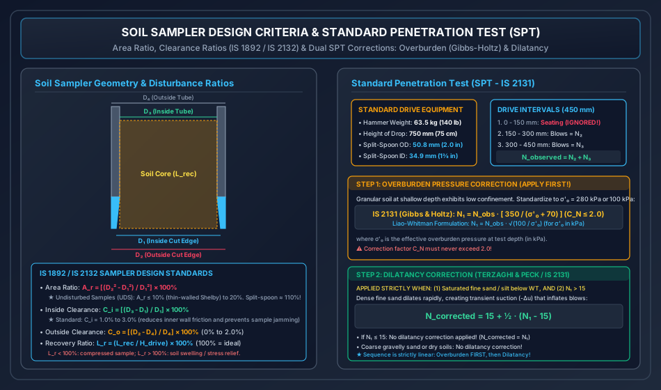
Sampler Design Geometrical Parameters (IS 1892 / IS 2132):
Let the dimensions of the sampling tool be:
- : Inside diameter of cutting edge / shoe.
- : Outside diameter of cutting edge / shoe.
- : Inside diameter of sampling tube.
- : Outside diameter of sampling tube.
1. Area Ratio ():
Measures the volume of soil displaced by the sampler walls during penetration relative to the sample core volume:
- For Undisturbed Soil Sampling (UDS): The area ratio must be kept as small as structurally possible:
- Thin-walled Shelby tubes: (mandatory for highly sensitive clays).
- Thick-walled samplers with cutting edge: .
- Standard split-spoon sampler ():
2. Inside Clearance Ratio ():
Allows the soil core to expand slightly elastically upon entering the tube, reducing internal frictional drag and preventing sample jamming:
- Standard Code Requirement: (typically ).
- If is too small: soil jams in the tube, causing severe compression.
- If is too large: sample slips out during withdrawal, and lateral expansion destroys structural fabric.
3. Outside Clearance Ratio ():
Reduces frictional drag on the external surface of the sampler tube during driving:
- Standard Code Requirement: (typically ).
4. Recovery Ratio ():
The ratio of the recovered core length to the actual penetration distance of the sampler:
- (): Good, undisturbed sample recovery.
- (): Sample suffered compression/compaction during driving.
- (): Sample expanded, swelled due to stress relief, or loose washings entered the tube.
5. Standard Penetration Test (SPT - IS 2131:1981)
The Standard Penetration Test (SPT) is the most widely utilized in-situ dynamic test for evaluating the density, shear strength, and allowable bearing pressure of cohesionless soils.
Standard Test Specifications (IS 2131):
- Drive Hammer: Drop weight of ().
- Height of Free Fall: Exactly ().
- Split-Spoon Sampler: Outside diameter (), inside diameter ().
Test Execution Procedure:
- Borehole is cleaned to the desired test depth.
- The split-spoon sampler attached to drill rods is lowered to the bottom of the borehole.
- The hammer is dropped repeatedly from height.
- Penetration is recorded in three consecutive () increments (total drive ):
- First : Regarded as the Seating Drive to bypass bottom disturbance and drilling mud washings. BLOWS ARE DISREGARDED!
- Second & Third : Blow counts (for ) and (for ) are recorded.
- The observed SPT -value is:
6. Dual Corrections to Observed SPT -Value
The raw observed blow count is subject to systematic field errors and MUST ALWAYS be corrected in a strictly sequential two-stage process:
Step 1: Overburden Pressure Correction ():
In cohesionless soils, confining pressure increases with depth. A loose sand at great depth can exhibit a higher blow count than a dense sand near the ground surface. To eliminate this confining bias, all blow counts are normalized to a standard effective overburden stress:
1. IS 2131 / Gibbs & Holtz Formulation (Standardized to or ):
- is the effective vertical overburden stress at the test depth in ().
- Upper Bound Limitation: The correction factor is strictly capped: .
- If , no overburden correction is applied ().
2. Liao & Whitman / ASTM D1586 Formulation (Normalized to ):
Step 2: Dilatancy (Water Table) Correction ():
Developed by Terzaghi and Peck (1948), this correction accounts for transient dynamic suction.
Mandatory Application Conditions:
The dilatancy correction is applied ONLY IF BOTH of the following conditions are simultaneously met:
- The subsoil stratum is saturated fine sand or silty sand located below the groundwater table.
- The overburden-corrected blow count exceeds 15 ().
Physical Rationale:
Dense, fine saturated sands dilate (expand) rapidly under dynamic hammer impact. Low permeability prevents pore water from rushing in instantly, inducing negative excess pore water pressures (suction, ). This transient suction momentarily increases effective stress (), artificially inflating the blow count.
Terzaghi & Peck Dilatancy Equation:
- If : No dilatancy correction is applied ().
- In coarse gravelly sands or dry soils above the water table: Dilatancy correction is NEVER applied.
┌────────────────────────────────────────────────────────────────────────────────────────────────────────┐
│                               CORRELATION OF SPT N-VALUE WITH SOIL PROPERTIES                          │
├──────────────────────────┬────────────────────────────┬─────────────────────────┬──────────────────────┤
│ Density State of Sand    │ Corrected SPT N-Value      │ Relative Density D_r (%)│ Friction Angle φ (°) │
├──────────────────────────┼────────────────────────────┼─────────────────────────┼──────────────────────┤
│ Very Loose               │ 0 - 4                      │ 0 - 15                  │ < 28°                │
│ Loose                    │ 4 - 10                     │ 15 - 35                 │ 28° - 30°            │
│ Medium Dense             │ 10 - 30                    │ 35 - 65                 │ 30° - 36°            │
│ Dense                    │ 30 - 50                    │ 65 - 85                 │ 36° - 42°            │
│ Very Dense               │ > 50                       │ > 85                    │ > 42°                │
└──────────────────────────┴────────────────────────────┴─────────────────────────┴──────────────────────┘
7. Cone Penetration Testing (CPT & CPTu Piezocone)
The Cone Penetration Test (CPT - IS 4968) provides continuous stratigraphical profiling without requiring a pre-drilled borehole.
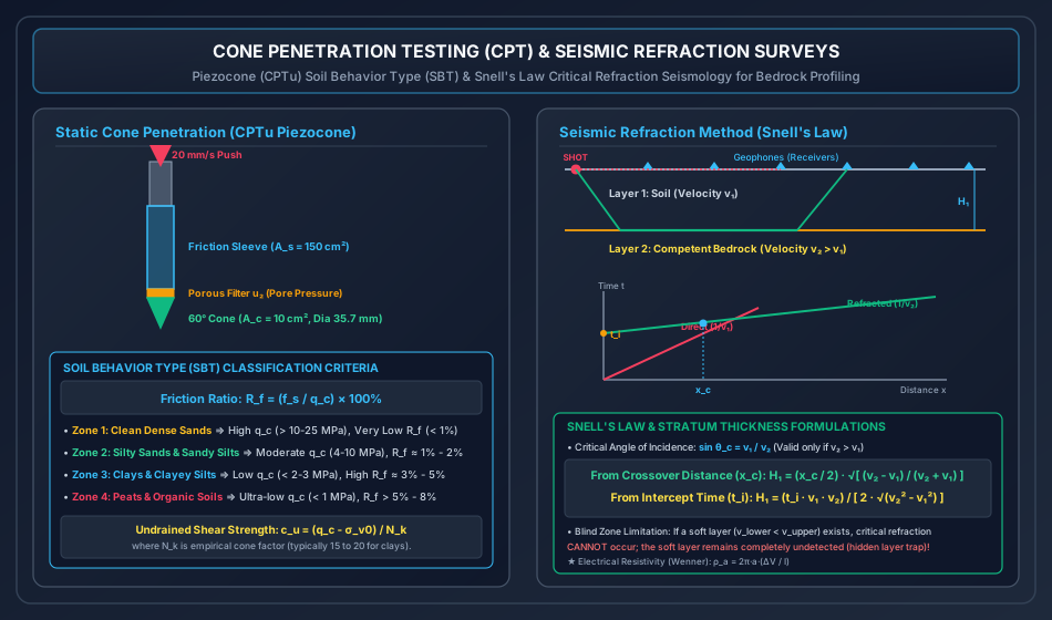
Mechanical & Electric Cone Specifications:
- Cone Tip: Apex angle , base projected area (diameter ).
- Friction Sleeve: Cylindrical surface area .
- Standard Penetration Rate: Pushed hydraulically at a constant rate of ().
Measured CPT Parameters:
- Cone Tip Resistance (): Total force on cone tip divided by base area: .
- Sleeve Friction (): Total skin friction on sleeve divided by sleeve area: .
- Friction Ratio ():
Soil Behavior Type (SBT) Classification:
- Clean Sands: High tip resistance (), very low friction ratio ().
- Silty Sands & Silts: Moderate tip resistance (), friction ratio .
- Cohesive Clays: Low tip resistance (), high friction ratio ().
- Organic Soils & Peats: Extremely low tip resistance (), very high friction ratio ().
Piezocone (CPTu) & Pore Pressure Transducer ():
A piezocone incorporates a porous stone filter (typically at the cone shoulder, position ) saturated with glycerin to measure dynamic pore water pressure during penetration:
- Corrected total cone resistance: , where is the net area ratio of the load cell.
- Undrained shear strength of clay from CPTu: where is the empirical cone factor ().
8. Geophysical Exploration: Seismic Refraction Method
Geophysical exploration provides rapid, non-destructive coverage over large construction sites. Among surface methods, seismic refraction is the standard technique for mapping bedrock topography.
Fundamental Physical Principle (Snell's Law):
Seismic waves generated by an impact hammer or explosive source travel through the upper stratum of velocity . At the interface with a denser lower stratum of velocity (), waves undergo refraction:
At the critical angle of incidence (), the refracted ray travels horizontally along the interface at the higher velocity ():
Time-Distance Relationship & Formulations:
Geophones placed along the ground surface record compressive -wave first arrivals:
- Direct Wave: Travels through the surface soil directly from source to geophone: Produces a straight line passing through the origin with slope .
- Critically Refracted Wave: Travels downward at angle , along the interface at , and upward at angle to the receiver: Produces a straight line with flatter slope and y-axis intercept time .
Depth to Bedrock ():
Method A: From Cross-over (Critical) Distance ():
The cross-over distance is the receiver distance where direct and refracted waves arrive at the exact same time ():
Method B: From Intercept Time ():
At , the refracted travel-time equation yields intercept :
The "Hidden Layer" / Blind Zone Limitation:
Seismic refraction operates strictly under the condition that velocity increases with depth (). If a softer, lower-velocity stratum exists beneath a dense crust (, e.g., soft clay underlying cemented sandstone):
- Waves refract toward the normal rather than along the boundary.
- No critical refraction occurs.
- The lower stratum remains completely invisible (hidden layer), leading to catastrophic misinterpretation of bedrock depth!
9. Electrical Resistivity Methods (Wenner & Schlumberger)
Electrical resistivity profiling detects variations in moisture content, soil salinity, and bedrock depths by injecting direct electric current () into the ground and measuring potential drop ().
Wenner Electrode Configuration:
Four collinear electrodes placed at equal spacing :
- Outer electrodes (): Current electrodes ().
- Inner electrodes (): Potential electrodes ().
where:
- is the apparent resistivity ().
- is the constant electrode spacing (m).
- is the measured voltage drop (V).
- is the injected direct current (A).
Profiling vs. Sounding:
- Resistivity Profiling (Trenching): Spacing is kept constant while the entire 4-electrode array is moved laterally across the site. Used to detect lateral geological faults, buried channels, and utility pipes.
- Resistivity Sounding (VES - Vertical Electrical Sounding): Center point remains fixed while electrode spacing is expanded incrementally. As spacing increases, current penetrates deeper into the ground, providing vertical stratification.
10. Subsoil Investigation Report (IS 1892)
A comprehensive geotechnical investigation culminates in a formal factual and interpretative Soil Investigation Report containing:
- Executive summary with clear foundation recommendations.
- Geological site overview and regional seismicity (IS 1893 Zone factor).
- Plan showing surveyed borehole locations, test pits, and geophysical lines.
- Borehole Logs: Visual soil description, layer boundaries, standard USCS/ISSCS symbols, groundwater table observations, raw and corrected SPT -values, sample extraction depths, and RQD.
- Laboratory test summary sheets (Atterberg limits, sieve curves, consolidation , triaxial Mohr envelopes).
- Engineering calculations for allowable bearing capacities (), group pile capacities, and predicted settlements ().
11. Solved Numerical Problems
Problem 1: Soil Sampler Geometry & Core Recovery Evaluation
Statement: A soil sampling tube equipped with a cutting shoe has the following measured dimensions:
- Cutting shoe inside diameter:
- Cutting shoe outside diameter:
- Sampling tube inside diameter:
- Sampling tube outside diameter:
During a sampling drive in a borehole, the sampler was driven a penetration distance of . The length of the soil sample recovered inside the tube was measured to be .
(a) Calculate the Area Ratio () of the sampler.
(b) Calculate the Inside Clearance Ratio ().
(c) Calculate the Outside Clearance Ratio ().
(d) Calculate the Recovery Ratio ().
(e) Evaluate whether this sampler satisfies IS 1892 / IS 2132 requirements for extracting undisturbed soil samples (UDS).
Solution:
Given: .
(a) Area Ratio ():
(b) Inside Clearance Ratio ():
(c) Outside Clearance Ratio ():
(d) Recovery Ratio ():
(e) Engineering Compliance Evaluation:
- Area Ratio: (and very close to the thin-wall limit).
- Inside Clearance: , which lies comfortably within the prescribed optimal range of .
- Outside Clearance: , which falls within .
- Recovery Ratio: , indicating minimal sample compression () and excellent core retention.
Problem 2: Standard Penetration Test Multi-Level Corrections
Statement: A Standard Penetration Test was conducted in a borehole drilled in a fine silty sand stratum below the groundwater table.
- Test depth in borehole:
- Depth of groundwater table: below ground level
- Bulk unit weight of soil above water table:
- Saturated unit weight of soil below water table:
The observed blow counts recorded for each of the three penetration drives were:
- to drive: blows
- to drive: blows
- to drive: blows
(a) Determine the raw observed SPT -value.
(b) Calculate the effective vertical overburden stress at the test depth.
(c) Compute the overburden correction factor and the overburden-corrected blow count using:
- (i) IS 2131 / Gibbs-Holtz equation
- (ii) Liao-Whitman equation
(d) Apply the dilatancy correction to obtain the final design SPT -value.
Solution:
(a) Raw Observed -value: The first is the seating drive and is disregarded:
(b) Effective Vertical Overburden Stress ():
- Soil above water table ( to ):
- Soil below water table ( to , thickness ):
- Total effective overburden stress at test depth :
(c) Overburden Pressure Correction ():
(i) IS 2131 / Gibbs & Holtz Method:
(Check: limit satisfied!)
(ii) Liao-Whitman Method:
(d) Dilatancy Correction (Terzaghi & Peck): Check criteria:
- Soil is saturated fine silty sand below the water table? YES ().
- Does ? YES ( for IS, and for Liao-Whitman).
Applying dilatancy correction:
-
Using IS 2131 Value ():
-
Using Liao-Whitman Value ():
Problem 3: Seismic Refraction Subsurface Layer Thickness Determination
Statement: A seismic refraction survey was conducted along a proposed viaduct alignment to map the depth to sound crystalline bedrock. First arrival times recorded by surface geophones yielded the following travel-time data:
- Compressional wave velocity in the topsoil layer:
- Compressional wave velocity in the underlying bedrock:
- The cross-over distance observed on the time-distance plot:
(a) Determine the critical angle of incidence () along the soil-rock interface.
(b) Calculate the thickness of the topsoil layer () using the cross-over distance formulation.
(c) Compute the intercept time () on the time axis and verify the calculated thickness .
Solution:
Given: .
(a) Critical Angle of Incidence (): According to Snell's Law:
(b) Layer Thickness () from Cross-over Distance ():
(c) Verification using Intercept Time ():
-
Theoretical intercept time:
-
Back-calculating from :
12. Comparative Engineering Analysis Across Syllabi
┌────────────────────────────────────────────────────────────────────────────────────────────────────────┐
│                        SYLLABUS EMPHASIS & EXAMINATION FOCUS MATRIX                            │
├─────────────┬─────────────────────────────────────────────────┬────────────────────────────────────────┤
│ Examination │ High-Yield Core Focus Areas                     │ Typical Question Typology              │
├─────────────┼─────────────────────────────────────────────────┼────────────────────────────────────────┤
│ GATE CE     │ • SPT dual corrections (overburden + dilatancy) │ 2-mark numericals on sequential SPT    │
│             │ • Sampler Area Ratio A_r & Inside Clearance C_i │ corrections; sampler clearance formulas;│
│             │ • Seismic refraction critical distance H_1      │ CPT friction ratio R_f calculations    │
├─────────────┼─────────────────────────────────────────────────┼────────────────────────────────────────┤
│ UPSC ESE    │ • Detailed boring methods and applicability     │ 10-15 mark conventional questions on   │
│             │ • Derivation of seismic refraction travel-time  │ UDS sampler criteria; Gibbs-Holtz vs   │
│             │ • Electrical resistivity Wenner array theory    │ Liao-Whitman; borehole logging details │
├─────────────┼─────────────────────────────────────────────────┼────────────────────────────────────────┤
│ SSC JE &    │ • SPT hammer weight 63.5 kg, fall 750 mm        │ Direct MCQs on seating drive (150 mm), │
│ RRB JE      │ • Area ratio limit A_r ≤ 10% for UDS            │ dilatancy formula 15 + 0.5(N-15);      │
│             │ • CPT cone angle 60°, base area 10 cm²          │ wash boring limitations                │
├─────────────┼─────────────────────────────────────────────────┼────────────────────────────────────────┤
│ State AE/JE │ • Lacey scour vs borehole exploration depth     │ Direct numerical substitutions of SPT  │
│             │ • RQD formula and rock quality rating table     │ corrections; RQD core recovery ratings │
└─────────────┴─────────────────────────────────────────────────┴────────────────────────────────────────┘
13. Common Misconceptions & Examination Pitfalls
-
Reversing the Order of SPT Corrections:
- Trap: Applying the dilatancy correction first, then the overburden correction.
- Reality: The sequence is strictly irreversible: Overburden correction MUST ALWAYS be applied first (), followed by Dilatancy correction (). Applying dilatancy first yields false, uncalibrated values!
-
Applying Dilatancy Correction in Dry or Coarse Soils:
- Trap: Applying in dry sand or gravel.
- Reality: Dilatancy suction requires saturation and low permeability (fine sands and silts). In coarse gravels or dry sands, water flows freely; zero suction develops. No dilatancy correction is permitted!
-
Including the First in SPT -Value:
- Trap: Summing all three drives: .
- Reality: The first drive is the seating drive to penetrate through loose sludge and disturbed bottom washings. It is strictly discarded: .
-
Blind Zone in Seismic Refraction:
- Trap: Assuming seismic refraction detects all geological layers.
- Reality: If a softer layer is sandwiched between stiffer layers (), Snell's law critical refraction cannot occur, making the soft layer completely invisible (hidden layer trap)!
-
Split-Spoon Sampler as Undisturbed Sampler:
- Trap: Calling split-spoon samples "undisturbed".
- Reality: The standard split-spoon sampler has . Split-spoon samples are highly disturbed representative samples, valid only for index property tests (Atterberg limits, sieve analysis).