Compressibility & 1D Consolidation Theory (Terzaghi), Settlement & Time Rate of Consolidation
In this chapter (8 topics)
On this page
- 1. Module Overview & Learning Objectives
- Core Exam Focus Areas
- 2. Consolidation Mechanics & Terzaghi's Spring-Piston Analogy
- The 4 Distinct Stages of Load Transfer
- 3. Mathematical Derivations & Compressibility Parameters
- 3.1 Fundamental 1D Strain-Void Ratio Relation
- 3.2 Coefficient of Compressibility (av)
- 3.3 Coefficient of Volume Compressibility (mv)
- 4. The e - logσ' Curve & Casagrande Preconsolidation Construction
- 4.1 Stress History Definitions
- 4.2 Casagrande's Empirical Construction for σp' (1936)
- 4.3 Compression Index (Cc) and Recompression Index (Cr)
- 5. Settlement Formulations: NC vs. OC Clays
- Case 1: Normally Consolidated Clay (σ0' = σp', OCR = 1.0)
- Case 2: Overconsolidated Clay with σ0' + Δσ' ≤ σp'
- Case 3: Overconsolidated Clay with σ0' < σp' < σ0' + Δσ'
- 6. Visual Master Diagram: 1D Consolidation Theory, Isochrones & Time Rate
- 7. Terzaghi's 1D Consolidation Theory
- 7.1 Assumptions of Terzaghi's Theory
- 7.2 Analytical Derivation of the Governing Equation
- 8. Drainage Boundary Conditions, Isochrones & Degree of Consolidation
- 8.1 Drainage Path Length (d)
- 8.2 Dimensionless Time Factor (Tv)
- 8.3 Average Degree of Consolidation (U)
- 9. Laboratory Oedometer Test & cv Curve Fitting Methods (IS 2720 Part 15)
- 9.1 Casagrande's Logarithm of Time Method (log t)
- 9.2 Taylor's Square Root of Time Method (√t)
- 10. Solved Numerical Problems (Step-by-Step, Pre-Calculated)
- Problem 1: Normally Consolidated vs. Overconsolidated Clay Settlement (GATE CE / UPSC ESE)
- Problem 2: Time Rate of Consolidation & Drainage Path Comparison (GATE CE / SSC JE)
- Problem 3: Oedometer Test Data Reduction & Hydraulic Conductivity (UPSC ESE)
- 11. Comparative Engineering Analysis & Multi-Exam Question Patterns
- 12. Common Misconceptions, Pitfalls & Pro-Tips
- Critical Traps to Avoid in Competitive Exams
- 13. Key Reference Formulas & Summary Table
1. Module Overview & Learning Objectives
When a structure (such as a high-rise building, bridge pier, embankment, or storage tank) is constructed upon a saturated clay deposit, the imposed foundation stresses create an immediate build-up of excess pore water pressure (). Because fine-grained clays possess exceptionally low hydraulic conductivities (), this excess pore water cannot escape instantaneously. As pore water slowly drains outward toward permeable boundary strata over months, years, or decades, load is transferred to the soil mineral skeleton, effective stress increases (), void ratio decreases, and the ground subsides. This hydrodynamic, time-dependent settlement process is termed Consolidation.
+----------------------------------------------------------------------------------------------------+
|                                  THE THREE STAGES OF SOIL SETTLEMENT                               |
+----------------------+----------------------+------------------------------------------------------+
| SETTLEMENT TYPE      | TIME DOMAIN          | PHYSICAL MECHANISM                                   |
+----------------------+----------------------+------------------------------------------------------+
| 1. Immediate /       | Immediate during     | Elastic distortion and lateral shearing of soil mass |
|    Elastic (S_i)     | construction         | at constant volume (undrained condition, Delta V = 0)|
+----------------------+----------------------+------------------------------------------------------+
| 2. Primary           | Time-dependent       | Hydrodynamic expulsion of pore water from voids;     |
|    Consolidation(S_c)| (months to decades)  | transfer of excess pore pressure to effective stress.|
+----------------------+----------------------+------------------------------------------------------+
| 3. Secondary         | Extremely slow       | Plastic creep, internal reorientation and structural |
|    Compression (S_s) | (continues after     | readjustment of clay platelets under constant        |
|                      | excess u = 0)        | effective stress (significant in organic soils/peat).|
+----------------------+----------------------+------------------------------------------------------+
Core Exam Focus Areas
- GATE CE: Exact computation of primary consolidation settlement () for Normally Consolidated (NC) and Overconsolidated (OC) clays; Preconsolidation pressure () and Overconsolidation Ratio (); 1D Terzaghi consolidation equation (); Time factor relations ( for , for ); Drainage path squaring rule ().
- UPSC ESE: Detailed derivation of Terzaghi's 1D consolidation differential equation from continuity and Darcy's law; Microscopic spring-piston analogy; Derivation of ; Casagrande log-time and Taylor square-root-of-time laboratory curve fitting procedures; Settlement calculation across split preconsolidation layers.
- SSC JE / State AE / RRB JE: Formula memory: , ; Skempton's empirical rule ; Double drainage () vs. single drainage ( longer); Standard milestone time factors (, ).
2. Consolidation Mechanics & Terzaghi's Spring-Piston Analogy
To elucidate the coupled physical interaction between fluid hydraulics and soil skeleton deformation, Karl Terzaghi (1925) introduced the classical Spring-Piston Hydrodynamic Model.
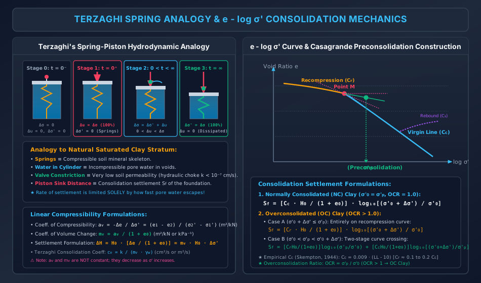
The 4 Distinct Stages of Load Transfer
-
Stage 0 (): Initial Unloaded State:
- The cylindrical vessel contains a compressible steel spring submerged in water. The drain valve is closed.
- Applied stress increment: .
- Excess pore water pressure: .
- Effective spring stress: .
-
Stage 1 (): Instantaneous Load Application (Valve Closed):
- An external vertical load is applied instantaneously to the piston. The escape valve remains tightly closed.
- Because water is practically incompressible compared to the metallic spring, water resists the entire load without permitting any piston movement.
- Excess pore pressure carries 100% of the load: .
- Effective spring stress is zero: . The spring undergoes zero compression.
-
Stage 2 (): Hydrodynamic Consolidation Phase (Valve Opened):
- The valve is opened. Under the driving head of excess pore pressure , water squirts out of the cylinder.
- As water escapes, the piston slowly descends, compressing the spring.
- Load is progressively transferred from the escaping pore water to the compressing spring:
- With increasing time: monotonically decays toward , while monotonically rises toward .
-
Stage 3 (): Complete Dissipation / Hydrodynamic Equilibrium:
- Outflow ceases entirely. Excess pore water pressure is completely dissipated: .
- The spring carries 100% of the applied load: .
- The piston reaches its maximum downward displacement, representing the ultimate primary consolidation settlement ().
+------------------------------------+---------------------------------------------------------------+
| MODEL ELEMENT                      | NATURAL CLAY PROTOTYPE COUNTERPART                            |
+------------------------------------+---------------------------------------------------------------+
| Compressible Steel Spring          | Deformable solid mineral soil skeleton                        |
| Water in Cylinder                  | Incompressible pore fluid filling void spaces                 |
| Constricted Escape Valve           | Extremely low permeability of clay (k < 10^-7 cm/s)           |
| Piston Downward Displacement       | Foundation consolidation settlement (S_c)                     |
+------------------------------------+---------------------------------------------------------------+
3. Mathematical Derivations & Compressibility Parameters
3.1 Fundamental 1D Strain-Void Ratio Relation
Consider a prism of saturated soil of initial height , solid height , and initial void ratio :
When subjected to a compressive effective stress increase , the height reduces by , while solid mineral height remains strictly invariant ():
Dividing by :
Therefore, the ultimate primary consolidation settlement is:
3.2 Coefficient of Compressibility ()
The coefficient of compressibility is defined as the decrease in void ratio per unit increase in effective pressure:
- Units: or (or ).
- Note: is not constant; it decreases markedly as effective stress increases because the soil skeleton stiffens.
3.3 Coefficient of Volume Compressibility ()
The coefficient of volume compressibility (or modulus of volume change) is the volumetric strain per unit increase in effective stress:
Substituting :
- Units: or .
- In terms of , consolidation settlement is directly expressed as:
4. The Curve & Casagrande Preconsolidation Construction
When void ratio is plotted against effective stress on a semi-logarithmic scale (), natural clays exhibit two distinct linear regimes separated by an inflection knee:
4.1 Stress History Definitions
- Preconsolidation Pressure ( or ): The maximum past effective vertical overburden stress that the soil deposit has ever experienced in its geological history.
- Current Overburden Stress (): The existing in-situ effective vertical overburden stress at the present day:
- Overconsolidation Ratio ():
- Normally Consolidated (NC) Clay (): The current effective stress is the maximum stress the soil has ever sustained ().
- Overconsolidated (OC) Clay (): The soil has experienced a past overburden stress greater than the current stress (), due to glacier retreat, geological erosion of overburden strata, or historic groundwater drawdowns.
- Underconsolidated Clay (): Soil deposit (such as recent deltaic or hydraulic land reclamation fill) that has not yet reached equilibrium under its own submerged weight and is currently consolidating.
4.2 Casagrande's Empirical Construction for (1936)
Arthur Casagrande formulated an exact graphical procedure to extract from an experimental oedometer curve:
- Locate the point of maximum curvature (minimum radius of curvature) on the curve, denoted as point .
- Draw a horizontal line passing through point .
- Draw a tangent line to the curve at point .
- Construct the bisector line of the angle formed between the horizontal line and the tangent line.
- Extend the lower straight-line portion (the Virgin Compression Curve) backward up to intersect the bisector line.
- The abscissa of this intersection point defines the Preconsolidation Pressure ().
4.3 Compression Index () and Recompression Index ()
-
Compression Index (): The slope of the linear virgin compression curve:
Skempton's Empirical Correlation for Normally Consolidated Clays (1944):
(For remolded clays: ).
-
Recompression / Swelling Index ( or ): The slope of the recompression curve during reloading or the rebound curve during unloading:
5. Settlement Formulations: NC vs. OC Clays
Consolidation settlement calculation depends strictly on the relation between the initial effective stress (), the preconsolidation pressure (), and the final stress ():
Case 1: Normally Consolidated Clay (, )
The entire load increment acts along the steep virgin compression curve ():
Case 2: Overconsolidated Clay with
The entire stress increment remains within the recompression zone; the past preconsolidation pressure is not exceeded. Settlement is small and governed solely by :
Case 3: Overconsolidated Clay with
The stress path crosses the preconsolidation pressure threshold. The settlement must be calculated in two separate stages:
- Recompression stage from to along slope .
- Virgin compression stage from to along slope .
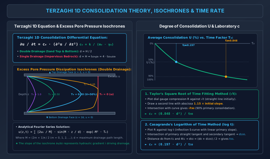
6. Visual Master Diagram: 1D Consolidation Theory, Isochrones & Time Rate
The following architectural diagram illustrates the derivation of Terzaghi's 1D consolidation differential equation, the spatial dissipation of excess pore water pressure across double-drainage isochrones, the average degree of consolidation () vs. time factor () curve, and standard laboratory curve fitting methods.
7. Terzaghi's 1D Consolidation Theory
7.1 Assumptions of Terzaghi's Theory
- The soil mass is homogeneous, isotropic, and completely saturated ().
- Both soil mineral grains and pore water are virtually incompressible.
- Flow of pore water is 1-dimensional (vertical only); lateral strain is zero (confined 1D strain).
- Darcy's law holds valid throughout the consolidation process ().
- The coefficient of permeability () and coefficient of volume compressibility () remain constant throughout the load increment.
- There is a unique, linear relationship between void ratio and effective stress ().
- Secondary compression and creep are neglected.
7.2 Analytical Derivation of the Governing Equation
Consider a soil element of cross-sectional area and thickness :
- By Darcy's law, upward inflow velocity at elevation is:
- Outflow velocity at elevation is:
- Net volumetric rate of water expulsion from element is:
By mass continuity, this rate of volume loss must equal the time rate of volumetric compression of the element:
Where volumetric strain is . Since total stress is constant during consolidation:
Therefore:
Equating the rate of volume change to the net seepage outflow:
Rearranging yields Terzaghi's 1D Consolidation Equation:
Where is the Coefficient of Consolidation:
- Dimensions:
- Units: or (or ).
8. Drainage Boundary Conditions, Isochrones & Degree of Consolidation
8.1 Drainage Path Length ()
The maximum distance that an expelled pore water droplet must travel to reach a permeable, free-draining boundary is the drainage path length ():
- Double Drainage (Open Layer): Sand strata exist both above and below the clay layer of total thickness :
- Single Drainage (Half-Closed Layer): Sand stratum exists on one face, while impervious rock/hard clay exists on the other:
8.2 Dimensionless Time Factor ()
The mathematical solution to Terzaghi's differential equation is parameterized by the dimensionless Time Factor:
The Fundamental Inverse-Square Law of Consolidation: For a given degree of consolidation ():
Comparing single drainage to double drainage for identical clay thickness :
A clay layer with single drainage requires four times as long to consolidate as an identical layer with double drainage!
8.3 Average Degree of Consolidation ()
The average degree of consolidation across the entire clay layer thickness at elapsed time is:
The mathematical relationship between and is expressed by two standardized analytical equations:
- For ():
- For ():
+------------------------------------+------------------------------------+
| DEGREE OF CONSOLIDATION (U %)      | TIME FACTOR (T_v)                  |
+------------------------------------+------------------------------------+
| 0%                                 | 0.0000                             |
| 10%                                | 0.0079                             |
| 20%                                | 0.0314                             |
| 30%                                | 0.0707                             |
| 40%                                | 0.1257                             |
| 50% (Crucial Milestone)            | 0.1964 (often taken as 0.197)      |
| 60%                                | 0.2827                             |
| 70%                                | 0.4030                             |
| 80%                                | 0.5670                             |
| 90% (Crucial Milestone)            | 0.8480                             |
| 95%                                | 1.1290                             |
| 100%                               | Infinity (Asymptotic)              |
+------------------------------------+------------------------------------+
9. Laboratory Oedometer Test & Curve Fitting Methods (IS 2720 Part 15)
In an oedometer (one-dimensional consolidation apparatus), a circular undisturbed soil specimen ( diameter, initial thickness) is placed in a rigid metal ring between porous stones and subjected to doubling incremental vertical loads ().
9.1 Casagrande's Logarithm of Time Method ()
- Plot dial gauge readings against . The curve forms an S-shaped inflection curve.
- Locate the theoretical primary consolidation point (): Select an early time on the initial parabolic curve, and another point at . The vertical distance between these points equals the distance between and .
- Locate the theoretical primary consolidation point (): Find the intersection of the tangent to the straight-line primary consolidation portion with the tangent to the final secondary compression tail.
- Calculate . The corresponding time is .
- Calculate :
9.2 Taylor's Square Root of Time Method ()
- Plot dial gauge readings against . The early portion of the curve is a straight line.
- Extend this straight line to intersect the deformation axis at .
- Draw a second straight line from having abscissae equal to times the abscissae of the first line.
- The intersection of this -slope line with the experimental curve defines the point.
- Square the value to get . Calculate :
10. Solved Numerical Problems (Step-by-Step, Pre-Calculated)
Problem 1: Normally Consolidated vs. Overconsolidated Clay Settlement (GATE CE / UPSC ESE)
A proposed building foundation imposes a uniform net effective stress increase of at the mid-depth of a thick saturated clay layer. The initial effective overburden stress at mid-depth is . Geotechnical laboratory tests on undisturbed specimens established:
- Initial void ratio
- Compression index
- Recompression index
Calculate the ultimate primary consolidation settlement () for three distinct geological histories:
- Case A: The clay is Normally Consolidated ().
- Case B: The clay is Overconsolidated with a past preconsolidation pressure .
- Case C: The clay is heavily Overconsolidated with .
Solution:
Given:
Case A: Normally Consolidated Clay () The entire stress increase lies on the virgin compression curve:
Case B: Overconsolidated Clay with Here, . The stress path crosses the preconsolidation threshold:
-
Recompression portion ():
-
Virgin portion ():
Case C: Heavily Overconsolidated Clay with Here, . The entire stress increment lies entirely on the recompression curve:
Problem 2: Time Rate of Consolidation & Drainage Path Comparison (GATE CE / SSC JE)
A saturated compressible clay layer of thickness has a coefficient of consolidation .
- If the clay is bounded by permeable sand layers at both top and bottom (Double Drainage):
- Determine the time required for consolidation () and consolidation () in days and years.
- Calculate the average degree of consolidation achieved after .
- If the clay is bounded by permeable sand at the top and impermeable bedrock at the bottom (Single Drainage):
- Calculate the time required for and consolidation.
Solution:
Part 1: Double Drainage ()
-
For :
-
For :
-
Degree of consolidation after ():
Since ():
Part 2: Single Drainage () Since , the time required is longer:
Problem 3: Oedometer Test Data Reduction & Hydraulic Conductivity (UPSC ESE)
In an oedometer consolidation test on a saturated clay specimen (, double drainage), the effective pressure was increased from to . The following observations were recorded:
- Void ratio at :
- Void ratio at :
- Time required for primary consolidation:
Determine:
- The coefficient of compressibility ().
- The coefficient of volume compressibility ().
- The coefficient of consolidation ().
- The hydraulic conductivity () of the clay specimen in and .
Solution:
Step 1: Coefficient of Compressibility ()
Step 2: Coefficient of Volume Compressibility ()
Step 3: Coefficient of Consolidation () Specimen thickness . Under double drainage:
Step 4: Hydraulic Conductivity () From Terzaghi's identity :
Substituting in consistent SI units ( in , in , ):
11. Comparative Engineering Analysis & Multi-Exam Question Patterns
+------------------------------------+-------------------------------------------------------------------------------------------------------------------+
| EXAM LEVEL                         | HIGHEST YIELD TOPICS & TYPICAL QUESTION PATTERNS                                                                 |
+------------------------------------+-------------------------------------------------------------------------------------------------------------------+
| GATE CE                            | - 2-stage settlement calculation for OC clay where stress increment crosses $\sigma_p'$.                          |
|                                    | - Time calculation scaling: $t_1 / t_2 = (d_1 / d_2)^2$ and $T_v = \frac{\pi}{4} U^2$.                             |
|                                    | - Extraction of $k$ from consolidation parameters ($k = c_v m_v \gamma_w$).                                       |
|                                    | - Identification of preconsolidation pressure via Casagrande graphical tangents.                                  |
+------------------------------------+-------------------------------------------------------------------------------------------------------------------+
| UPSC ESE                           | - Analytical derivation of Terzaghi's 1D consolidation differential equation.                                     |
|                                    | - Complete tabular comparison between Spring Analogy and natural clay consolidation.                              |
|                                    | - Taylor $\sqrt{t}$ ($1.15$ slope) vs. Casagrande $\log t$ ($d_0 - d_{50} - d_{100}$) fitting procedures.           |
|                                    | - Secondary compression index ($C_\alpha = \Delta e / \Delta\log_{10} t$) and creep settlement calculation.        |
+------------------------------------+-------------------------------------------------------------------------------------------------------------------+
| SSC JE / RRB JE                    | - Direct settlement formula: $\Delta H = H \frac{\Delta e}{1+e_0} = m_v H \Delta\sigma'$.                        |
|                                    | - Single vs double drainage time ratio ($t_{\text{single}} = 4 \times t_{\text{double}}$).                        |
|                                    | - Skempton formula: $C_c = 0.009(LL - 10)$.                                                                       |
|                                    | - Milestone values: $T_{v,50} \approx 0.197$, $T_{v,90} \approx 0.848$.                                           |
+------------------------------------+-------------------------------------------------------------------------------------------------------------------+
| State AE / JE                      | - Definitions of NC, OC, and Underconsolidated soils ($OCR = \sigma_p' / \sigma_0'$).                             |
|                                    | - Units of $a_v$ and $m_v$ ($\text{m}^2/\text{kN}$) and $c_v$ ($\text{cm}^2/\text{s}$).                           |
|                                    | - Assumption validity: $S = 100\%$, 1D strain, valid Darcy law.                                                   |
+------------------------------------+-------------------------------------------------------------------------------------------------------------------+
12. Common Misconceptions, Pitfalls & Pro-Tips
Critical Traps to Avoid in Competitive Exams
- The Drainage Path Halving Trap ( vs ):
- For double drainage: .
- For single drainage: .
- Students frequently forget to square the ratio, writing instead of .
- The Denominator Trap: In the settlement equations: Always use the initial void ratio () in the denominator, never the final void ratio () or average void ratio.
- OC Clay Two-Stage Split: When calculating settlement for an overconsolidated clay where , you cannot compute the entire settlement with . You must split the calculation at : use from to , and use from to . Using for the whole increment grossly overestimates settlement.
- Time Factor Validity Thresholds:
- Use strictly for .
- For , the parabolic formula underestimates ; use the logarithmic formula .
- Units Consistency in : If is in and is in or , you must convert to () and use to obtain in . Mixing and is the #1 source of numerical errors in GATE!
13. Key Reference Formulas & Summary Table
+-------------------------------------------------------+-------------------------------------------------------------+
| PARAMETER / FORMULA                                   | MATHEMATICAL EXPRESSION                                     |
+-------------------------------------------------------+-------------------------------------------------------------+
| Primary Consolidation Settlement (Void Ratio)         | S_c = H_0 * [Delta_e / (1 + e_0)]                           |
+-------------------------------------------------------+-------------------------------------------------------------+
| Primary Consolidation Settlement (Volume Change)      | S_c = m_v * H_0 * Delta_sigma'                              |
+-------------------------------------------------------+-------------------------------------------------------------+
| Primary Settlement (NC Clay, OCR = 1.0)               | S_c = [C_c * H_0 / (1 + e_0)] * log10[(sigma_0' + Delta_sigma') / sigma_0'] |
+-------------------------------------------------------+-------------------------------------------------------------+
| Primary Settlement (OC Clay, sigma_f' <= sigma_p')     | S_c = [C_r * H_0 / (1 + e_0)] * log10[(sigma_0' + Delta_sigma') / sigma_0'] |
+-------------------------------------------------------+-------------------------------------------------------------+
| Primary Settlement (OC Clay, sigma_0' < sigma_p' < sigma_f') | S_c = [C_r * H_0 / (1 + e_0)] * log10(sigma_p' / sigma_0') |
|                                                       |     + [C_c * H_0 / (1 + e_0)] * log10(sigma_f' / sigma_p')  |
+-------------------------------------------------------+-------------------------------------------------------------+
| Overconsolidation Ratio                               | OCR = sigma_p' / sigma_0'                                   |
+-------------------------------------------------------+-------------------------------------------------------------+
| Empirical Compression Index (Skempton)                | C_c = 0.009 * (LL - 10)                                     |
+-------------------------------------------------------+-------------------------------------------------------------+
| Coefficient of Compressibility                        | a_v = -Delta_e / Delta_sigma'  (m^2/kN)                     |
+-------------------------------------------------------+-------------------------------------------------------------+
| Coefficient of Volume Compressibility                 | m_v = a_v / (1 + e_0)  (m^2/kN or kPa^-1)                   |
+-------------------------------------------------------+-------------------------------------------------------------+
| Terzaghi 1D Consolidation Differential Equation       | du/dt = c_v * (d^2 u / dz^2)                                |
+-------------------------------------------------------+-------------------------------------------------------------+
| Coefficient of Consolidation                          | c_v = k / (m_v * gamma_w)  (cm^2/s or m^2/s)                |
+-------------------------------------------------------+-------------------------------------------------------------+
| Time Factor                                           | T_v = (c_v * t) / d^2                                       |
+-------------------------------------------------------+-------------------------------------------------------------+
| Time Factor for U <= 60%                              | T_v = (pi / 4) * (U / 100)^2                                |
+-------------------------------------------------------+-------------------------------------------------------------+
| Time Factor for U > 60%                               | T_v = 1.781 - 0.933 * log10(100 - U%)                       |
+-------------------------------------------------------+-------------------------------------------------------------+
| Key Time Factor Milestones                            | T_v,50 = 0.197 (U = 50%),  T_v,90 = 0.848 (U = 90%)         |
+-------------------------------------------------------+-------------------------------------------------------------+
| Drainage Ratio Law                                    | t_single = 4 * t_double  (for identical layer thickness H)  |
+-------------------------------------------------------+-------------------------------------------------------------+
| Casagrande Fitting Formula (Log t)                    | c_v = (0.197 * d^2) / t_50                                  |
+-------------------------------------------------------+-------------------------------------------------------------+
| Taylor Fitting Formula (Sqrt t)                       | c_v = (0.848 * d^2) / t_90                                  |
+-------------------------------------------------------+-------------------------------------------------------------+
Authored with mathematical rigor, IS code precision (IS 2720 Part 15), and multi-exam alignment for the Civil Engineering Academic Knowledge Repository.