Soil Compaction, Standard & Modified Proctor Tests, OMC, MDD, Field Rollers & Quality Control
In this chapter (8 topics)
On this page
- 1. Module Overview & Learning Objectives
- Core Exam Focus Areas
- 2. Fundamental Principles & Physics of Compaction
- The Lubrication Theory (R.R. Proctor, 1933)
- 3. Mathematical Derivations & Analytical Formulations
- 3.1 Bulk Unit Weight and Dry Unit Weight
- 3.2 Dry Density as a Function of Degree of Saturation (S)
- 3.3 Theoretical Zero Air Void Line (ZAVL)
- 3.4 Dry Density as a Function of Percentage Air Voids (na)
- 4. Visual Master Diagram: Proctor Compaction Curves & ZAVL
- Essential Diagram Key Takeaways
- 5. Standard Proctor vs. Modified Proctor Tests (IS 2720 Part 7 & Part 8)
- 5.1 Exact Compaction Energy Calculation
- 6. Soil Microstructure & Engineering Properties: Dry vs. Wet of Optimum
- 6.1 Lambe's Double-Layer Evolution
- 6.2 Engineering Property Comparison: Dry vs. Wet of Optimum
- 7. Field Compaction Equipment & Roller Selection Matrix
- 8. Field Quality Control & Density Determination
- 8.1 In-Situ Density Test Methods
- 9. Solved Numerical Problems (Step-by-Step, Pre-Calculated)
- Problem 1: Standard Proctor Test Data Reduction, OMC & Air Voids (GATE CE / UPSC ESE)
- Problem 2: Field Quality Control via Sand Replacement Method (GATE CE / SSC JE)
- Problem 3: Compaction Energy Ratio & Compactive Effort Mechanics (UPSC ESE / State AE)
- 10. Comparative Engineering Analysis & Multi-Exam Question Patterns
- 11. Common Misconceptions, Pitfalls & Pro-Tips
- Critical Traps to Avoid in Competitive Exams
- 12. Key Reference Formulas & Summary Table
1. Module Overview & Learning Objectives
Soil compaction is an artificial mechanical process by which soil grains are rearranged into a more dense configuration by the dynamic application of mechanical energy (rolling, tamping, or vibrating), resulting in the expulsion of air voids with little to no immediate change in water content. Unlike consolidation (which is a slow, time-dependent expulsion of pore water under sustained static load), compaction is an instantaneous mechanical process that drastically improves engineering performance:
- Increases shear strength and bearing capacity.
- Decreases compressibility and post-construction settlement.
- Drastically reduces hydraulic conductivity (permeability), preventing seepage piping and internal erosion.
- Mitigates frost heave and moisture susceptibility in subgrades and embankments.
+----------------------------------------------------------------------------------------------------+
|                                    SOIL COMPACTION FOUNDATIONS                                     |
+------------------------------------+---------------------------------------------------------------+
| COMPACTION (Mechanical Process)    | CONSOLIDATION (Hydrodynamic Process)                          |
+------------------------------------+---------------------------------------------------------------+
| Expulsion of pore AIR              | Expulsion of pore WATER                                       |
| Instantaneous (seconds to minutes) | Time-dependent (months to centuries)                          |
| Dynamic mechanical energy applied  | Static sustained overburden load                              |
| Soil partially saturated (S < 100%)| Soil fully saturated (S = 100%)                               |
| Dry density gamma_d increases      | Void ratio e decreases under effective stress increase        |
+------------------------------------+---------------------------------------------------------------+
Core Exam Focus Areas
- GATE CE: Theoretical derivation of Zero Air Void Line (ZAVL) and Air Voids lines (); line of optimums; compactive effort shifts; Lambe's microstructural evolution (dry vs. wet of OMC); exact calculation of relative compaction (), air void ratio (), and saturation () at maximum dry density (MDD).
- UPSC ESE: Detailed comparison of IS light compaction (IS 2720 Part 7) vs. IS heavy compaction (IS 2720 Part 8); Proctor mold dimensions, rammer weights, free drop heights, and layer counts; roller mechanisms and suitability matrix (sheepsfoot vs. smooth vs. pneumatic vs. vibratory).
- SSC JE / State AE / RRB JE: Formula memory (, ); Proctor test specifications (2.6 kg / 310 mm drop vs. 4.9 kg / 450 mm drop); sand replacement vs. core cutter suitability (core cutter cannot be used in stony/gravelly soils).
2. Fundamental Principles & Physics of Compaction
The Lubrication Theory (R.R. Proctor, 1933)
When dry soil is subjected to mechanical compaction, high interparticle friction resists grain rearrangement, yielding a relatively low dry density. As water is incrementally introduced:
- Lubrication Stage (Dry of Optimum): Thin water films envelop soil particles, acting as a lubricant. Interparticle friction is significantly reduced, enabling the applied dynamic impact to slide soil particles into tighter, more compact packing arrangements. Bulk density and dry density rise steadily with increasing water content .
- Peak Density (Optimum Moisture Content - OMC): At a critical moisture content, water films attain optimum lubrication efficiency without occupying excessive pore space. The dry density reaches its mathematical maximum ( or MDD).
- Displacement Stage (Wet of Optimum): Past the OMC, water possesses negligible compressibility. Excess water begins to displace solid soil particles within the fixed volume of the compaction mold. Because the density of water () is far lower than the density of mineral soil solids (), the dry unit weight falls precipitously.
       Dry Density gamma_d
               ^
               |               Peak = MDD
               |                 * (OMC, MDD)
               |               /   \
               |              /     \    Compaction Curve
               |  Lubrication/       \   Displacement Zone
               |  Zone      /         \  (Water displaces solids)
               |           /           \
               |          /             \
               +---------------------------------> Water Content w (%)
                                  OMC
3. Mathematical Derivations & Analytical Formulations
3.1 Bulk Unit Weight and Dry Unit Weight
From the definition of phase parameters:
Since water content is :
In terms of mass density:
3.2 Dry Density as a Function of Degree of Saturation ()
Starting from basic phase relations:
Using the identity :
3.3 Theoretical Zero Air Void Line (ZAVL)
The Zero Air Void Line represents the absolute theoretical upper bound of compaction where the degree of saturation is () and air content , volume of air :
Critical Law: In actual field or laboratory dynamic compaction, it is physically impossible to expel 100% of entrapped air pockets. Consequently, no practical soil compaction curve can ever cross, touch, or lie above the Zero Air Void Line. The compaction curve always peaks and drops strictly to the left and below the ZAVL.
3.4 Dry Density as a Function of Percentage Air Voids ()
The percentage air voids is defined as the volume of air per total soil volume :
The total volume is partitioned as:
Dividing by :
Expressing solid and water volumes in terms of mass and unit weights:
Substituting into the expression for :
Rearranging for dry unit weight :
GATE Trap Alert: Note the critical distinction between (percentage air voids ) and (air content ). When using , the formula contains in the numerator:
When using , the formula is:
These two formulations are mathematically equivalent because .
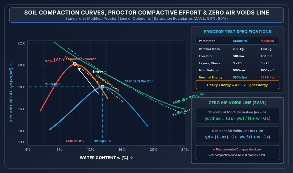
4. Visual Master Diagram: Proctor Compaction Curves & ZAVL
The following architectural diagram illustrates the experimental compaction curves obtained under Standard Proctor and Modified Proctor efforts, the shift in Optimum Moisture Content (OMC) and Maximum Dry Density (MDD), the line of optimums, and the theoretical bounding Zero Air Void Line.
Essential Diagram Key Takeaways
- Compactive Effort Shift: Increasing the compactive effort (Modified vs. Standard) shifts the compaction curve upward and to the left:
- Maximum Dry Density increases ().
- Optimum Moisture Content decreases ().
- Line of Optimums: The locus connecting the peak points of compaction curves obtained at different compactive efforts runs nearly parallel to the Zero Air Void Line (). It never intersects the ZAVL.
- High Water Content Convergence: At high water contents (far wet of optimum), the curves for different compactive efforts merge into a single curve asymptotic to the ZAVL. At such excessive water contents, higher mechanical energy cannot displace more air because pores are already filled with incompressible water.
5. Standard Proctor vs. Modified Proctor Tests (IS 2720 Part 7 & Part 8)
The standard laboratory tests quantify the relationship between moisture content and dry unit weight under standardized mechanical compaction energies.
+------------------------------------+------------------------------------+------------------------------------+
| PARAMETER                          | STANDARD PROCTOR / IS LIGHT        | MODIFIED PROCTOR / IS HEAVY        |
|                                    | (IS 2720 Part 7 : 1980)            | (IS 2720 Part 8 : 1983)            |
+------------------------------------+------------------------------------+------------------------------------+
| Internal Diameter of Mold         | 100 mm                             | 100 mm                             |
| Height of Mold                     | 127.3 mm                           | 127.3 mm                           |
| Mold Volume (V)                    | 1000 cm^3 (1.0 litre)              | 1000 cm^3 (1.0 litre)              |
| Mass of Compaction Rammer (M)      | 2.60 kg                            | 4.90 kg                            |
| Free Drop Height of Rammer (H)     | 310 mm (31.0 cm)                   | 450 mm (45.0 cm)                   |
| Number of Soil Layers (N_L)        | 3 layers                           | 5 layers                           |
| Blows per Layer (N_B)              | 25 blows                           | 25 blows                           |
| Total Compaction Energy per Volume | 593.0 kJ/m^3                       | 2697.8 kJ/m^3                      |
| Energy Multiplication Factor       | 1.00x (Baseline)                   | 4.55x                              |
| Typical Field Applications         | Retaining wall backfills, light    | Modern expressways, heavy aircraft |
|                                    | embankments, small earthen dams    | runways, high-speed rail subgrade  |
+------------------------------------+------------------------------------+------------------------------------+
5.1 Exact Compaction Energy Calculation
The mechanical work done per unit volume of soil is given by:
-
For IS Light Compaction (Standard Proctor):
-
For IS Heavy Compaction (Modified Proctor):
-
Energy Ratio:
6. Soil Microstructure & Engineering Properties: Dry vs. Wet of Optimum
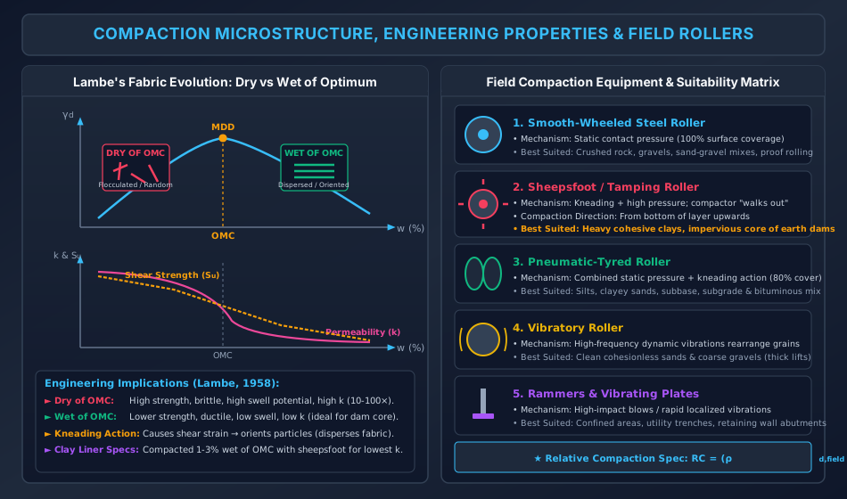
T.W. Lambe (1958) formulated the classical microstructural theory of compacted cohesive soils based on Gouy-Chapman diffuse double layer theory.
6.1 Lambe's Double-Layer Evolution
- Dry of Optimum ():
- Water is scarce; the electrolyte concentration in pore water is high.
- The electric diffuse double layer surrounding clay platelets is severely depressed (very thin double layer).
- Interparticle repulsive forces () are negligible; van der Waals attractive forces () strongly dominate.
- When compacted, particles lock into an edge-to-face random, flocculated fabric.
- Wet of Optimum ():
- High water content dilutes electrolyte concentration, expanding the diffuse double layer.
- Net interparticle repulsion () forces clay platelets to glide past each other under compaction shearing.
- Particles align into a face-to-face parallel, dispersed fabric.
6.2 Engineering Property Comparison: Dry vs. Wet of Optimum
+------------------------------------+------------------------------------+------------------------------------+
| ENGINEERING PROPERTY               | COMPACTED DRY OF OPTIMUM           | COMPACTED WET OF OPTIMUM           |
+------------------------------------+------------------------------------+------------------------------------+
| Soil Fabric / Particle Orientation | Flocculated (Random edge-to-face)  | Dispersed (Parallel face-to-face)  |
| Hydraulic Conductivity (k)         | High (inter-aggregate macro-pores) | Low (10x to 100x lower than dry)   |
| Shear Strength (Undrained)         | Significantly Higher               | Lower                              |
| Stress-Strain Behavior             | Brittle (sharp post-peak drop)     | Ductile (plastic, large strain)    |
| Pore Water Pressure at Failure     | Low or negative (dilatant tendency)| High positive pore water pressure  |
| Swelling Potential (on wetting)    | High (particles want to disperse)  | Low (already expanded)             |
| Shrinkage Potential (on drying)    | Low (random fabric resists volume) | High (parallel platelets collapse) |
| Compressibility under Low Stress   | Very low                           | Higher                             |
| Compressibility under High Stress  | Higher (flocculated bonds collapse)| Lower                              |
| Recommended Practical Application | Highway subgrades, foundation fills| Impervious core of earth dams,     |
|                                    | requiring high bearing strength    | hazardous waste clay liners        |
+------------------------------------+------------------------------------+------------------------------------+
7. Field Compaction Equipment & Roller Selection Matrix
Proper selection of compaction plant is dictated by soil type, gradation, plasticity, layer lift thickness, and project specifications.
+------------------------------------+------------------------------------+------------------------------------+
| EQUIPMENT TYPE                     | DOMINANT COMPACTION MECHANISM      | BEST SUITED SOIL & FIELD USAGE     |
+------------------------------------+------------------------------------+------------------------------------+
| 1. Smooth-Wheeled Steel Rollers    | Static pressure; 100% ground       | Crushed stones, gravels, well-     |
|    (8 to 12 tonnes)                | contact area; contact stress up to | graded sands. Finishing & proof    |
|                                    | 300 - 400 kPa.                     | rolling of subgrade surfaces.      |
+------------------------------------+------------------------------------+------------------------------------+
| 2. Sheepsfoot / Tamping Rollers    | Kneading action + high contact     | Heavy cohesive clays, impervious   |
|    (Feet project 15-25 cm from     | pressure (up to 1400 - 7000 kPa);  | core of earth dams. Compaction     |
|    drum surface; 8-12% contact)    | "walks out" of layer from bottom.  | proceeds from bottom upwards.      |
+------------------------------------+------------------------------------+------------------------------------+
| 3. Pneumatic-Tyred Rollers         | Static pressure + kneading action  | Silts, clayey sands, sandy gravels,|
|    (Rubber tyres with variable     | (80% ground contact area; tyre     | highway subbase and bituminous     |
|    inflation pressure 200-700 kPa) | pressure 600 - 800 kPa).           | carpet finishing.                  |
+------------------------------------+------------------------------------+------------------------------------+
| 4. Vibratory Rollers               | High-frequency dynamic vibrations  | Clean cohesionless sands, gravels, |
|    (Steel drum with internal       | (1000 - 3000 vpm) breaking grain-  | rockfill dams. Highly effective in |
|    eccentric eccentric masses)     | to-grain interlocking.             | thick lifts (up to 1.0 m).         |
+------------------------------------+------------------------------------+------------------------------------+
| 5. Impact Rammers & Tampers        | Dynamic impact blows / localized   | Confined spaces, narrow utility    |
|    (Manual pneumatic/electric)     | rapid vibration plate.             | trenches, bridge abutment backfills|
+------------------------------------+------------------------------------+------------------------------------+
Roller Operation Rule (Exam Golden Rule): Sheepsfoot rollers compact from the bottom of the layer upwards. As the soil compacts, the feet penetrate less and less until the roller "walks out" to the surface. Smooth-wheeled rollers compact from the top downwards.
8. Field Quality Control & Density Determination
Field compaction control requires verifying that the in-situ dry density meets the design relative compaction criteria:
8.1 In-Situ Density Test Methods
1. Core Cutter Method (IS 2720 Part 29)
- Apparatus: Cylindrical steel cutter ( internal diameter, height, volume) driven into ground with steel rammer () and dolly.
- Bulk Density:
- Dry Density:
- Limitations: Strictly limited to soft, fine-grained, cohesive soils without gravel. Cannot be used in stony, gravelly, or dry cohesionless sands (driving damages the cutter or fails to retain sand).
2. Sand Replacement Method (IS 2720 Part 28)
- Apparatus: Sand pouring cylinder with conical shutter; calibrated clean uniform standard sand passing and retained on sieve.
- Steps:
- Determine bulk density of calibrated sand: .
- Excavate a test hole of diameter equal to cylinder hole ( or , depth ). Weigh excavated wet soil ().
- Place pouring cylinder over hole, open shutter. Sand fills hole and cone.
- Mass of sand in hole: .
- Volume of excavated hole: .
- Field bulk density: .
- Field dry density: .
- Suitability: Universal method applicable to all soils (cohesive, coarse gravelly, hard soils).
3. Water Displacement Method
- Used for cohesive, clayey undisturbed lumps coated with molten paraffin wax.
4. Nuclear Density Gauge
- Emits gamma radiation (Cesium-137) for bulk density and neutron moderation (Americium-241/Beryllium) for moisture content. Rapid non-destructive test.
9. Solved Numerical Problems (Step-by-Step, Pre-Calculated)
Problem 1: Standard Proctor Test Data Reduction, OMC & Air Voids (GATE CE / UPSC ESE)
A laboratory Standard Proctor compaction test was performed on a clayey silt soil with using a mold (). The test data recorded are:
+------------+----------------------+--------------------+
| Point No.  | Water Content w (%)  | Total Mass (g)     |
+------------+----------------------+--------------------+
| 1          | 8.5                  | 2860               |
| 2          | 11.0                 | 2980               |
| 3          | 13.5                 | 3050               |
| 4          | 16.0                 | 3020               |
| 5          | 18.5                 | 2940               |
+------------+----------------------+--------------------+
Determine:
- The Maximum Dry Density (MDD in ) and Optimum Moisture Content (OMC in ) by parabolic fitting around the peak.
- The void ratio (), degree of saturation (), and percentage air voids () at the optimum state.
- The theoretical Zero Air Void dry density at the OMC.
Solution:
Step 1: Compute bulk density and dry unit weight for each trial For each trial, mass of wet soil . With :
- Point 1 ():
- Point 2 ():
- Point 3 ():
- Point 4 ():
- Point 5 ():
Step 2: Parabolic peak determination (Points 2, 3, 4) Fitting through points , , gives:
Solving gives the exact parabolic vertex coordinates:
Step 3: State parameters at MDD ()
-
Void ratio ():
-
Degree of saturation ():
-
Percentage air voids ():
-
Zero Air Void dry density at OMC ():
Notice:
Problem 2: Field Quality Control via Sand Replacement Method (GATE CE / SSC JE)
A highway embankment is being compacted with a specification requiring a minimum relative compaction of of laboratory MDD (). Quality control testing by the sand replacement method gave the following observations:
- Bulk density of calibrated Ottawa sand:
- Mass of sand filling the cone alone:
- Initial mass of sand in cylinder:
- Final mass of sand in cylinder after filling excavated hole and cone:
- Mass of wet soil excavated from hole:
- Moisture content of excavated soil:
Determine:
- The volume of the excavated test hole ().
- The field in-situ dry density ( and ).
- The Relative Compaction () achieved, and whether the field compaction meets the technical specification.
Solution:
Step 1: Calculate mass of sand filling the excavated hole
Step 2: Calculate volume of excavated hole
Step 3: Field bulk density and dry density
Step 4: Relative Compaction () and Specification Check
Problem 3: Compaction Energy Ratio & Compactive Effort Mechanics (UPSC ESE / State AE)
Calculate the total compaction energy per cubic metre imparted in the Indian Standard Light Compaction test (IS 2720 Part 7) versus the Indian Standard Heavy Compaction test (IS 2720 Part 8), using standard specifications:
- Light Compaction: Rammer mass , drop height , , , mold volume .
- Heavy Compaction: Rammer mass , drop height , , , mold volume .
Find the multiplication factor by which energy is increased, and explain the structural effect of this increase on the position of the compaction curve.
Solution:
Step 1: Energy in IS Light Compaction
Step 2: Energy in IS Heavy Compaction
Step 3: Ratio of Compactive Energies
Step 4: Structural Effect on Compaction Curve With a -fold increase in compactive effort:
- The compaction curve moves upward ( increases by typically ).
- The compaction curve shifts leftward ( decreases by typically ).
- The peak point moves along the Line of Optimums, which is roughly parallel to the Zero Air Void Line.
10. Comparative Engineering Analysis & Multi-Exam Question Patterns
+------------------------------------+-------------------------------------------------------------------------------------------------------------------+
| EXAM LEVEL                         | HIGHEST YIELD TOPICS & TYPICAL QUESTION PATTERNS                                                                 |
+------------------------------------+-------------------------------------------------------------------------------------------------------------------+
| GATE CE                            | - Numerical computation of $S$, $e$, $n_a$ at MDD from Proctor test data.                                         |
|                                    | - ZAVL equation verification ($\gamma_d = G_s\gamma_w / (1 + w G_s)$).                                           |
|                                    | - Microstructural contrast: dry of optimum vs wet of optimum permeability and swelling behavior.                |
|                                    | - Line of optimums characteristics and non-intersection with ZAVL.                                               |
+------------------------------------+-------------------------------------------------------------------------------------------------------------------+
| UPSC ESE                           | - Derivation of $\gamma_d = (1-n_a)G_s\gamma_w / (1 + w G_s)$ from first principles.                            |
|                                    | - Full tabular specification comparison of IS 2720 Part 7 (Light) vs Part 8 (Heavy).                            |
|                                    | - Detailed engineering justification for equipment selection (e.g., why Sheepsfoot roller is required for clay). |
|                                    | - Proctor needle penetrometer calibration for rapid field moisture estimation.                                    |
+------------------------------------+-------------------------------------------------------------------------------------------------------------------+
| SSC JE / RRB JE                    | - Direct formula questions: $\gamma_d = \gamma / (1 + w)$.                                                        |
|                                    | - Weight of Proctor hammer ($2.6\text{ kg}$ Light, $4.9\text{ kg}$ Heavy).                                       |
|                                    | - Free fall drop height ($31\text{ cm}$ Light, $45\text{ cm}$ Heavy).                                             |
|                                    | - Layer counts ($3\text{ layers}$ Light, $5\text{ layers}$ Heavy).                                                |
|                                    | - Roller matching: Sheepsfoot → Clay; Vibratory → Sand; Pneumatic → Base/subgrade.              |
+------------------------------------+-------------------------------------------------------------------------------------------------------------------+
| State AE / JE                      | - Core cutter applicability criteria (only fine-grained cohesive soils; unsuitable for gravelly/sandy soil).      |
|                                    | - Relative compaction definition ($RC = \rho_{d,\text{field}} / \rho_{d,\text{lab}} \times 100\%$).              |
|                                    | - Effect of adding compaction energy on OMC and MDD.                                                             |
+------------------------------------+-------------------------------------------------------------------------------------------------------------------+
11. Common Misconceptions, Pitfalls & Pro-Tips
Critical Traps to Avoid in Competitive Exams
- ZAVL Intersection Error: No compaction curve can cross or even touch the Zero Air Void Line. In multiple-choice questions, any diagram showing a curve crossing the ZAVL is physically invalid.
- Air Voids () vs Air Content ():
- Percentage air voids: . Formula: .
- Air content: . Formula: .
- Confusing with leads to massive numerical errors in GATE!
- Core Cutter Misapplication: Core cutter method is strictly for soft cohesive soils. Never select core cutter for gravelly subgrades or clean dry sands because pebbles damage the cutter edge and dry sands will not stay inside the cutter during extraction.
- Energy Scaling Myth: Modifying the Proctor test does not just increase MDD; it decreases OMC. Many students erroneously assume that higher energy requires more water. Higher energy packs grains tighter, requiring less water for particle lubrication.
- Dam Core Compaction Rule: The impervious clay core of an earthen dam should always be compacted slightly wet of optimum ( to wet of OMC) using a sheepsfoot roller. Why? Because wet compaction yields a dispersed fabric that minimizes hydraulic conductivity () and eliminates brittle cracking, accommodating differential settlement safely.
12. Key Reference Formulas & Summary Table
+-------------------------------------------------------+-------------------------------------------------------------+
| PARAMETER / FORMULA                                   | MATHEMATICAL EXPRESSION                                     |
+-------------------------------------------------------+-------------------------------------------------------------+
| Dry Unit Weight from Bulk Weight                      | gamma_d = gamma / (1 + w)                                   |
+-------------------------------------------------------+-------------------------------------------------------------+
| Dry Density with Saturation (S)                       | gamma_d = (G_s * gamma_w) / [1 + (w * G_s) / S]             |
+-------------------------------------------------------+-------------------------------------------------------------+
| Zero Air Void Line (ZAVL, S = 100%, n_a = 0)          | gamma_d,ZAVL = (G_s * gamma_w) / (1 + w * G_s)              |
+-------------------------------------------------------+-------------------------------------------------------------+
| Dry Density with Percentage Air Voids (n_a)           | gamma_d = [(1 - n_a) * G_s * gamma_w] / (1 + w * G_s)      |
+-------------------------------------------------------+-------------------------------------------------------------+
| Air Void Ratio - Saturation Identity                  | n_a = n * a_c = [e / (1 + e)] * (1 - S)                     |
+-------------------------------------------------------+-------------------------------------------------------------+
| Standard Proctor Energy per Volume                    | E_std = (2.60 kg * 9.81 * 0.310 m * 3 * 25) / 10^-3 m^3     |
|                                                       |        = 593.01 kJ/m^3                                      |
+-------------------------------------------------------+-------------------------------------------------------------+
| Modified Proctor Energy per Volume                    | E_mod = (4.90 kg * 9.81 * 0.450 m * 5 * 25) / 10^-3 m^3     |
|                                                       |        = 2703.88 kJ/m^3  (4.56x E_std)                      |
+-------------------------------------------------------+-------------------------------------------------------------+
| Relative Compaction (RC)                              | RC = [gamma_d(field) / gamma_d(lab_MDD)] * 100%             |
+-------------------------------------------------------+-------------------------------------------------------------+
| Field Density (Sand Replacement)                      | V_hole = M_sand_hole / rho_sand                             |
|                                                       | rho_field = M_wet_soil / V_hole                             |
+-------------------------------------------------------+-------------------------------------------------------------+
Authored with mathematical rigor, IS code precision (IS 2720 Part 7 & Part 8), and multi-exam alignment for the Civil Engineering Academic Knowledge Repository.