Gradually Varied Flow (GVF): Governing Differential Equation, Slope Classifications, 12 Surface Water Profiles & Direct Step Method
In this chapter (4 topics)
On this page
- 1. Module Overview & Pedagogical Scope
- 2. Official Examination Syllabus Mapping
- 3. Fundamental Physical Principles & Governing Assumptions
- 3.1 Slope Definitions & Energy Gradients
- 3.2 Channel Bed Slope Classification
- 3.3 The Three Depth Zones
- 4. Mathematical Derivations & Rigorous Proofs
- Proof 1: Derivation of the GVF Dynamic Differential Equation
- Proof 2: Wide Rectangular Channel Power-Law Formulation
- Proof 3: Analytical Derivation of the 12 Surface Water Profiles
- Proof 4: Boundary Asymptotes & Singularity Conditions
- Proof 5: The Direct Step Numerical Integration Method
- 5. Technical Diagrams & Interactive Architectural Schematics
- Diagram 1: GVF Slope Classification & Depth Zones
- Diagram 2: The 12 Water Surface Profiles & Hydraulic Transitions
- 6. Comparative Engineering Analysis & Parameter Regimes
- Table 6.1: Complete Classification Matrix of the 12 GVF Water Surface Profiles
- 7. Worked Numerical Examples (Pre-Calculated & Verified)
- Problem 1: GVF Profile Identification & Slope Classification
- Problem 2: Direct Step Backwater Computation Behind a Dam (M1 Curve)
- Problem 3: Multi-Slope Transition & Profile Synthesis
- 8. High-Yield Examination Traps & Ambiguities
- Trap 1: The Three Non-Existent GVF Profiles (C2, H1, A1)
- Trap 2: Profile Slopes at Boundary Lines (dy/dx at NDL and CDL)
- Trap 3: Sign of dy/dx Across Zones
- Trap 4: Direction of Direct Step Computation
- 9. Real-World Engineering Applications & Case Studies
- 9.1 Reservoir Backwater & Flood Inundation Modeling (Bhakra Dam)
- 9.2 Highway Culvert Tailwater & Drop Inlets
- 10. Cross-Disciplinary & Downstream Dependencies
- 11. Summary Formula Cheat Sheet & Memory Anchors
- 12. Comprehensive References & Standard Codes
1. Module Overview & Pedagogical Scope
Gradually Varied Flow (GVF) is defined as steady non-uniform open channel flow in which the water depth and velocity vary gradually along the longitudinal channel distance . Unlike Rapidly Varied Flow (RVF, such as hydraulic jumps or flow over sharp-crested weirs) where streamline curvature is pronounced and vertical accelerations cannot be neglected, in GVF:
- The curvature of the streamlines is so gentle that the vertical acceleration of fluid particles is negligible ().
- The pressure distribution across any vertical section is strictly hydrostatic ().
- The channel is assumed to be prismatic with a constant longitudinal bed slope .
- The true rate of energy dissipation per unit length (the friction slope ) at any section is assumed to be identical to the friction slope of a uniform flow having the same cross-sectional area, velocity, hydraulic radius, and roughness ().
The fundamental objective of GVF analysis is to predict the longitudinal water surface profile created by natural boundary transitions and artificial hydraulic structures (dams, barrages, sluice gates, culvert entrances, drops, and changes in channel bed slope).
2. Official Examination Syllabus Mapping
Website note: this mapping is from the author’s notes. It has not been checked against the official notification for each examination; confirm the current syllabus with the examining body.
| Examination Body | Primary Syllabus Line | Recurring Problem Archetypes |
|---|---|---|
| GATE CE | Gradually varied flow, dynamic equation, classification of surface water profiles, direct step method. | • Derivation of the dynamic equation . • Identification of active profile type (, etc.) given boundary controls. • Numerical computation of backwater curve reach length using the Direct Step Method. |
| UPSC ESE | Fluid Mechanics & Hydraulics: Non-uniform flow, GVF profiles, controls, backwater computation. | • Qualitative profiling through series channel transitions (Mild Steep, Steep Mild with jump). • Asymptotic boundary conditions: Why curves strike CDL vertically and approach NDL asymptotically. • Proof that , and profiles cannot physically exist. |
| SSC JE / RRB JE | Hydraulics: Classification of slopes, types of water surface profiles. | • Criteria for Mild (), Steep (), Critical (). • Sign of across Zone 1 (+ve, rising), Zone 2 (-ve, falling), Zone 3 (+ve, rising). |
| State AE / JE | Water Resources & Irrigation Engineering: Reservoir backwater and flood inundation. | • Calculation of submergence length upstream of a barrage or check dam. |
3. Fundamental Physical Principles & Governing Assumptions
3.1 Slope Definitions & Energy Gradients
In the analysis of open channel transitions, three distinct longitudinal slopes govern the kinematics:
- Bed Slope (): Rate of fall of the channel invert datum:
- Water Surface Slope (): Rate of fall of the piezometric hydraulic grade line:
- Energy Slope / Friction Slope (): Rate of total mechanical energy dissipation per unit length:
- In Uniform Flow: Bed, water surface, and energy lines are parallel:
- In Gradually Varied Flow: The slopes diverge:
3.2 Channel Bed Slope Classification
Channel bed slopes are classified into five distinct regimes based on the relative magnitude of the Normal Depth () (governed by Manning's uniform flow equation) versus the Critical Depth () (governed by Froude critical energy minimization):
- Mild Slope (): (). Uniform flow is subcritical ().
- Steep Slope (): (). Uniform flow is supercritical ().
- Critical Slope (): (). Normal depth equals critical depth; uniform flow is critical ().
- Horizontal Bed (): . Bed slope is zero, implying normal depth is infinite ().
- Adverse Slope (): . The bed rises in the direction of flow. Steady uniform flow cannot exist ( is imaginary).
3.3 The Three Depth Zones
Each channel slope profile is partitioned into three vertical depth zones bounded by the Normal Depth Line (NDL) and the Critical Depth Line (CDL):
- Zone 1: Flow depth lies above both NDL and CDL ( and ). Flow is subcritical.
- Zone 2: Flow depth lies between NDL and CDL ( or ).
- Zone 3: Flow depth lies below both NDL and CDL ( and ). Flow is supercritical.
4. Mathematical Derivations & Rigorous Proofs
Proof 1: Derivation of the GVF Dynamic Differential Equation
Consider a reach of an open channel with total energy head :
Assuming the kinetic energy correction factor :
-
Differentiating with Respect to Longitudinal Distance :
-
Applying the Chain Rule to the Velocity Head:
Since (surface top width):
-
Substituting Slope Definitions: Recall that and :
-
Rearranging for Longitudinal Depth Gradient :
(The fundamental dynamic equation of Gradually Varied Flow!).
-
Alternative Formulation in Terms of Specific Energy : Since :
Since , the equation naturally recurs.
Proof 2: Wide Rectangular Channel Power-Law Formulation
For a wide rectangular channel where width , the hydraulic radius is approximately equal to depth: , and .
-
Expressing in Terms of Depth Ratio (): From Manning's equation for uniform flow:
For varied flow at depth :
Dividing by :
-
Expressing Froude Number in Terms of Critical Depth Ratio ():
-
Substituted Wide Channel Dynamic Equation:
where hydraulic exponents are and . (If Chezy's formula is utilized, , yielding Bresse's classical analytical integration equation).
Proof 3: Analytical Derivation of the 12 Surface Water Profiles
The sign of dictates whether the water depth increases in the direction of flow (backwater / rising curve, ) or decreases (drawdown / falling curve, ).
1. Mild Slope Profiles ():
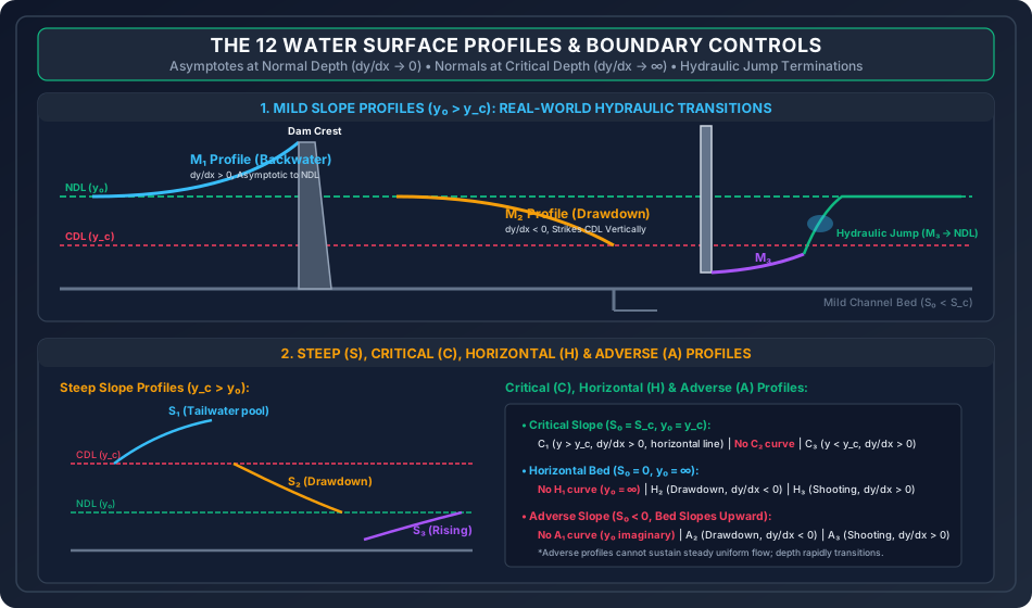
- Profile (Zone 1: ):
- (Numerator ).
- (Denominator ).
- (Rising / Backwater Curve).
- Occurrence: Upstream of a dam, weir, or barrage in a natural river.
- Profile (Zone 2: ):
- (Numerator ).
- (Denominator ).
- (Drawdown Curve).
- Occurrence: Approaching a sudden channel drop, free overfall, or entrance into a steep chute.
- Profile (Zone 3: ):
- Numerator .
- Denominator .
- (Rising Curve).
- Occurrence: Supercritical flow emerging from beneath a sluice gate onto a mild channel; rises rapidly until terminating in a hydraulic jump.
2. Steep Slope Profiles ():
- Profile (Zone 1: ):
- Numerator , Denominator (Rising Curve).
- Occurrence: Flow on a steep slope submerged by a high downstream tailwater weir.
- Profile (Zone 2: ):
- Numerator , Denominator (Drawdown Curve).
- Occurrence: Downstream of a slope break from mild to steep; draws down to .
- Profile (Zone 3: ):
- Numerator , Denominator (Rising Curve).
- Occurrence: Sluice gate outflow on a steep slope rising asymptotically to .
3. Critical Slope Profiles ():
- Profile (Zone 1: ): (Rises as a horizontal line).
- Profile (Zone 3: ): (Rises towards critical depth).
- Non-Existence of Profile: Because , there is zero physical space between NDL and CDL. Flow at is uniform critical flow, possessing a perfectly horizontal free surface parallel to the bed.
4. Horizontal Bed Profiles ():
Since , :
- Profile (): (Drawdown Curve).
- Profile (): (Rising Curve).
- Non-Existence of : Since , flow depth cannot exceed infinity.
5. Adverse Slope Profiles ():
Since , is strictly negative:
- Profile (): (Drawdown Curve).
- Profile (): (Rising Curve).
- Non-Existence of : is mathematically imaginary.
Proof 4: Boundary Asymptotes & Singularity Conditions
-
Asymptotic Approach to the Normal Depth Line (NDL): As , the actual velocity and hydraulic radius approach uniform flow values. Thus, .
Theorem: All GVF curves approach the Normal Depth Line tangentially and asymptotically ().
-
Perpendicular Intersection with the Critical Depth Line (CDL): As , . The denominator vanishes:
Theorem: Theoretically, all GVF curves intersect the Critical Depth Line vertically (at to the bed). (Physical Reality: When becomes large, vertical streamline curvature violates GVF assumptions, transforming the flow into a rapid wave, undular jump, or standing surge).
-
Approach to Infinite Depth (): As , and :
Recall that water surface slope is . As , . Theorem: At very large depths (deep reservoir pool), the water surface becomes completely horizontal.
Proof 5: The Direct Step Numerical Integration Method
For prismatic channels of known geometry, distance can be integrated directly as a function of depth steps :
-
Energy Conservation Between Sections 1 and 2 separated by distance :
Since :
-
Solving for Step Distance :
where the mean friction slope over the step is arithmetic:
- If computation proceeds upstream (as in subcritical flow profiles ): .
- If computation proceeds downstream (as in supercritical flow profiles ): .
5. Technical Diagrams & Interactive Architectural Schematics
Diagram 1: GVF Slope Classification & Depth Zones
+--------------------------------------------------------------------------------------------------+
| FIGURE 1: THE 5 BED SLOPES (M, S, C, H, A) & DEPTH REGIME SIGNAGE MATRIX                        |
+--------------------------------------------------------------------------------------------------+
The schematic below maps out the relative positioning of the Normal Depth Line (NDL) and Critical Depth Line (CDL) across Mild, Steep, Critical, Horizontal, and Adverse slopes, indicating the signage of across Zones 1, 2, and 3.
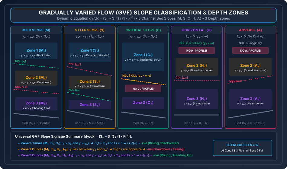
Diagram 2: The 12 Water Surface Profiles & Hydraulic Transitions
+--------------------------------------------------------------------------------------------------+
| FIGURE 2: THE 12 SURFACE PROFILES UNDER DAM BACKWATER, DROP OVERFALL & SLUICE CONTROLS           |
+--------------------------------------------------------------------------------------------------+
The schematic below details real-world boundary transitions including dam backwater curves (), free overfalls (), sluice gate outflows with hydraulic jumps (), steep slope transitions (), and asymptotic alignments.
6. Comparative Engineering Analysis & Parameter Regimes
Table 6.1: Complete Classification Matrix of the 12 GVF Water Surface Profiles
| Profile Code | Bed Slope Condition | Depth Range | Froude Number | Numerator () | Denominator () | Sign of | Nature of Surface Curve | Typical Engineering Occurrence |
|---|---|---|---|---|---|---|---|---|
| Mild () | + | + | +ve | Backwater (Rising) | Upstream of dam / barrage in natural river. | |||
| Mild () | - | + | -ve | Drawdown (Falling) | Approaching canal drop, sudden expansion, or weir. | |||
| Mild () | - | - | +ve | Backwater (Rising) | Supercritical flow under sluice gate into mild pool. | |||
| Steep () | + | + | +ve | Backwater (Rising) | Tailwater drowning on steep chute spillway. | |||
| Steep () | + | - | -ve | Drawdown (Falling) | Steep slope downstream of a break from mild grade. | |||
| Steep () | - | - | +ve | Backwater (Rising) | Flow below sluice gate discharging onto steep slope. | |||
| Critical () | + | + | +ve | Horizontal Line | Pool upstream of overflow structure on critical slope. | |||
| Critical () | — | — | — | — | — | DOES NOT EXIST | represents uniform critical flow. | |
| Critical () | - | - | +ve | Backwater (Rising) | Outflow from sluice gate on critical slope. | |||
| Horizontal () | — | — | — | — | — | DOES NOT EXIST | Normal depth . | |
| Horizontal () | - | + | -ve | Drawdown (Falling) | Flow in a flat canal approaching a free overfall. | |||
| Horizontal () | - | - | +ve | Backwater (Rising) | Sluice gate outflow discharging into flat canal. | |||
| Adverse () | — | — | — | — | — | DOES NOT EXIST | Normal depth is imaginary. | |
| Adverse () | - | + | -ve | Drawdown (Falling) | Flow rising over an adverse upward ramp. | |||
| Adverse () | - | - | +ve | Backwater (Rising) | Sluice gate jet shooting up an adverse slope. |
7. Worked Numerical Examples (Pre-Calculated & Verified)
Problem 1: GVF Profile Identification & Slope Classification
Problem Statement: A rectangular channel of width carries a steady discharge . The bed slope is () and Manning's roughness coefficient is .
- Compute the critical depth and normal depth .
- Classify the channel bed slope as Mild, Steep, or Critical.
- Determine the type of surface profile (, etc.), the Froude number , and the sign and magnitude of at:
- Flow depth
- Flow depth
- Flow depth
Step-by-Step Solution:
-
Critical Depth ():
-
Normal Depth (): From Manning's equation for uniform flow:
Solving iteratively via Newton-Raphson:
-
Slope Classification:
-
Surface Profile Evaluation at Specified Depths:
-
Case 1: Depth ():
(Positive gradient confirms is a rising backwater curve!).
-
Case 2: Depth ():
(Negative gradient confirms is a falling drawdown curve!).
-
Case 3: Depth ():
(Negative over negative yields positive; is a rising supercritical curve!).
-
Problem 2: Direct Step Backwater Computation Behind a Dam ( Curve)
Problem Statement: In the rectangular channel of Problem 1 (, normal depth ), a diversion weir backs up water to a depth immediately upstream of the structure. Using the Direct Step Method with depth increments of , determine the length of the backwater reach upstream of the dam to where the flow depth reduces to .
Step-by-Step Solution:
-
Step Discretization: We integrate upstream from the dam ( at ) across three successive stations:
- Station 0:
- Station 1:
- Station 2:
- Station 3:
-
Tabulated Direct Step Calculations:
| Step | Flow Depth (m) | Flow Area () | Velocity (m/s) | Specific Energy (m) | Friction Slope | Average | (m) | Step Length (m) | Cumulative Distance (m) |
|---|---|---|---|---|---|---|---|---|---|
| 0 | 2.80 | 14.00 | 1.0714 | 2.8585 | 0.000203 | — | — | — | 0.00 |
| 1 | 2.60 | 13.00 | 1.1538 | 2.6679 | 0.000247 | 0.000225 | -0.1907 | -1087.73 | -1087.73 |
| 2 | 2.40 | 12.00 | 1.2500 | 2.4796 | 0.000305 | 0.000276 | -0.1882 | -1517.84 | -2605.57 |
| 3 | 2.30 | 11.50 | 1.3043 | 2.3867 | 0.000342 | 0.000324 | -0.0929 | -1220.14 | -3825.71 |
-
Sample Detailed Calculation for Step 1 ():
- At : .
- At : .
- Mean friction slope: .
- Energy change: .
- Step distance:
-
Total Backwater Reach Length:
(The influence of the dam extends upstream over a length of before the depth drops back within of the natural uniform flow depth).
Problem 3: Multi-Slope Transition & Profile Synthesis
Problem Statement: A rectangular channel of width , discharge , and experiences an abrupt transition in longitudinal slope from an upstream mild slope () to a downstream steep slope ().
- Determine the critical depth and normal depths and on both reaches.
- Identify the specific GVF profile curves that develop upstream and downstream of the break in grade.
- Establish the location where critical depth occurs.
Step-by-Step Solution:
-
Hydraulic Regimes on Reaches:
- Critical depth: (governed strictly by and , independent of slope).
- Reach 1 (): Normal depth .
- Reach 2 (): Solve Manning's equation for : Solving iteratively:
-
Water Surface Profile Transitions:
- Upstream of Break (Mild Reach): Flow approaches from the deep subcritical normal depth . To enter the downstream steep slope, the water surface must draw down towards critical depth:
- Downstream of Break (Steep Reach): Flow enters the steep reach near critical depth and must accelerate down to the supercritical normal depth :
-
Location of Critical Depth (): The critical depth serves as the hydraulic control section. In reality, due to curvilinear flow, occurs a very short distance upstream (approximately ) of the break in slope, directly linking the curve to the curve without forming a hydraulic jump!
8. High-Yield Examination Traps & Ambiguities
[!WARNING]
Trap 1: The Three Non-Existent GVF Profiles ()
In competitive exams (GATE, ESE, State PSCs), questions frequently include bogus options featuring , or . Remember:
- No profile: On a critical slope, . Zone 2 has zero vertical thickness. Flow at is uniform critical flow.
- No profile: For a horizontal bed, . No flow can exist above infinite depth.
- No profile: For an adverse bed, is mathematically imaginary.
- Total number of real GVF profiles is exactly 12 ().
[!WARNING]
Trap 2: Profile Slopes at Boundary Lines ( at NDL and CDL)
- At the Normal Depth Line (NDL): . The surface profile is asymptotic / tangent to NDL.
- At the Critical Depth Line (CDL): . The surface profile theoretically strikes CDL vertically / perpendicularly.
[!WARNING]
Trap 3: Sign of Across Zones
You can instantly determine the sign of without memorizing formulas:
- All Zone 1 curves () have (Rising / Backwater curves).
- All Zone 2 curves () have (Falling / Drawdown curves).
- All Zone 3 curves () have (Rising curves).
[!CAUTION]
Trap 4: Direction of Direct Step Computation
- For Subcritical Flow Profiles (): Control is at the downstream boundary. Step calculations must proceed upstream ().
- For Supercritical Flow Profiles (): Control is at the upstream boundary. Step calculations must proceed downstream ().
9. Real-World Engineering Applications & Case Studies
9.1 Reservoir Backwater & Flood Inundation Modeling (Bhakra Dam)
When a large dam or barrage (such as Bhakra Dam on the Sutlej River or Sardar Sarovar Dam on the Narmada) impounds water, the water level at the reservoir structure is held high above normal river depth.
- An extensive backwater curve develops, extending tens of kilometers upstream into natural river valleys.
- Accurate GVF numerical modeling (using the Standard Step Method in software packages like HEC-RAS) is legally mandatory to establish the High Flood Level (HFL) and map upstream agricultural land acquisition boundaries, preventing unexpected flooding of upstream towns.
9.2 Highway Culvert Tailwater & Drop Inlets
When designing roadway drainage, culverts discharging onto steep downstream embankments create an drawdown profile that rapidly accelerates flow into high-velocity supercritical jets (). If unmitigated, this jet scours the downstream highway toe. Engineers must predict the profile to correctly size stilling basins and riprap protection aprons.
10. Cross-Disciplinary & Downstream Dependencies
                                    +-------------------------------------------------------------+
                                    |         OCF-03: GRADUALLY VARIED FLOW & PROFILES            |
                                    |         dy/dx = (S0 - Sf)/(1 - Fr^2), 12 Profiles           |
                                    +-------------------------------------------------------------+
                                                                   |
                                  +--------------------------------+--------------------------------+
                                  |                                                                 |
                                  v                                                                 v
+-----------------------------------------------------+   +-----------------------------------------------------+
|         OCF-04: RAPIDLY VARIED FLOW (RVF)           |   |       IRRI-03: CANAL REGULATORS & HEADWORKS         |
|   M3 Profile termination via Hydraulic Jump,        |   |   Afflux computation behind barrages, Backwater     |
|   Sequent depth matching (y_jump = y_sequent)       |   |   Inundation, Energy Dissipator Stilling Basins     |
+-----------------------------------------------------+   +-----------------------------------------------------+
- Downstream Module
OCF-04: Whenever a supercritical GVF profile ( or ) is forced to transition into a subcritical downstream pool, it cannot merge smoothly because at CDL. The GVF profile terminates abruptly in a Hydraulic Jump, where the post-jump sequent depth must match the downstream subcritical depth. - Irrigation Engineering (
IRRI-03): The height of guide banks and flood protection levees upstream of barrages is designed by adding freeboard to the computed backwater curve.
11. Summary Formula Cheat Sheet & Memory Anchors
| Entity | Primary Formula | Examination Mnemonic / Rule |
|---|---|---|
| GVF Dynamic Eq. | Net slope over Froude deficit | |
| Wide Channel Eq. | Exponents: (Manning) & (Froude) | |
| Energy Gradient | Bed slope minus friction slope | |
| Direct Step Length | Specific energy change over net slope | |
| Friction Slope | Manning's friction formula | |
| NDL Boundary | Asymptotic / tangent to NDL | |
| CDL Boundary | Vertical / normal to CDL | |
| Deep Pool Boundary | Water surface becomes horizontal | |
| Non-Existent Profiles | "Can't Have Adverse 1" (Only 12 real profiles) | |
| Zone Sign Rule | Zone 1: , Zone 2: , Zone 3: | 1 & 3 Rise, 2 Falls |
12. Comprehensive References & Standard Codes
- Subramanya, K. (2019). Flow in Open Channels, 5th Edition, McGraw-Hill Education, New Delhi. (Chapter 4: Gradually Varied Flow).
- Chow, Ven Te (1959). Open-Channel Hydraulics, McGraw-Hill Book Company, New York. (Chapter 8: Theoretical Analysis of GVF).
- Henderson, F. M. (1966). Open Channel Flow, Macmillan Publishing, New York.
- Bresse, J. A. C. (1860). Cours de Mécanique Appliquée, 2e partie, Hydraulique, Mallet-Bachelier, Paris. (Original analytical integration of backwater curves).
- Bureau of Indian Standards (BIS):
- IS 10430: 2000 — Criteria for Design of Lined Canals and Guidelines for Selection of Type of Lining.
- IS 6934: 1998 — Hydraulic Design of Groynes and Guide Banks in Alluvial Rivers.
- U.S. Army Corps of Engineers (USACE): HEC-RAS River Analysis System Hydraulic Reference Manual, Hydrologic Engineering Center, Davis, CA.