Abstractions from Precipitation: Evaporation, Transpiration, Evapotranspiration (PET/AET), Infiltration & Infiltration Indices (φ and W Index)
In this chapter (4 topics)
On this page
- 1. Module Scope & Pedagogical Objectives
- 2. Comprehensive Syllabus Mapping
- 3. Physical Principles, Thermodynamics & Hydrologic Abstractions
- 3.1 Thermodynamic Physics of Evaporation
- 3.2 Dalton’s Law of Evaporation (1802)
- 3.3 Transpiration & Evapotranspiration Regimes
- 3.4 Mechanics of Infiltration
- 4. Rigorous Mathematical Formulations & Analytical Derivations
- 4.1 Proof 1: Aerodynamic Evaporation Formulations (Meyer & Rohwer)
- 4.2 Proof 2: Penman’s Theoretical Equation for PET
- 4.3 Proof 3: Horton’s Infiltration Equation & Cumulative Integration
- 4.4 Proof 4: The Infiltration Indices (φ-Index & W-Index)
- 5. Hand-Coded High-Precision Engineering Visualizations
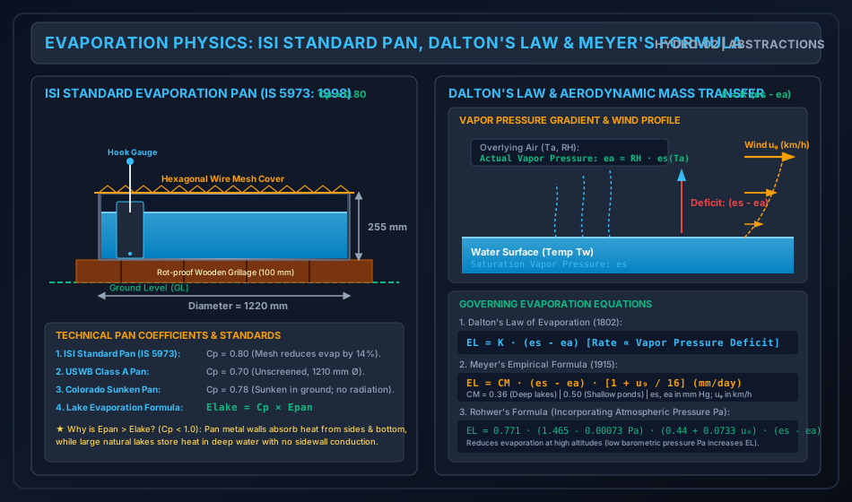
- 5.1 Diagram 1: Evaporation Physics, ISI Standard Pan & Meyer's Formulations
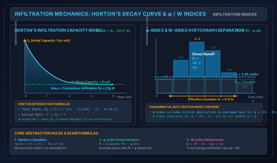
- 5.2 Diagram 2: Horton's Infiltration Curve & Hyetograph Partitioning by φ / W Indices
- 6. Comparative Engineering Analysis & Cross-Sectional Synthesis
- 6.1 Evaporation Measurement Equipment & Pan Characteristics
- 6.2 Major Mathematical Infiltration Models Comparison
- 7. Fully Worked Numerical Problems (Pre-Calculated & Verified)
- Problem 1: Reservoir Evaporation via Meyer’s Formula vs ISI Standard Pan
- Problem 2: Horton’s Infiltration Capacity Curve & Surface Runoff
- Problem 3: φ-Index and W-Index Determination from a Complex Hyetograph
- 8. Critical Exam Traps, Failure Modes & Conceptual Pitfalls
- 9. Real-World Engineering Case Studies & Forensic Failures
- 9.1 Reservoir Evaporation Mitigation in Aswan High Dam (Lake Nasser, Egypt)
- 9.2 Flash Flooding from Wildfire Hydrophobicity (California, USA)
- 10. Cross-Disciplinary & Downstream Dependencies
- 11. High-Yield Revision Formula Cheat Sheet
- 12. Authoritative References & Standards
1. Module Scope & Pedagogical Objectives
When atmospheric precipitation falls upon a natural drainage basin, only a fraction of the gross water depth is converted directly into surface streamflow. The remainder is consumed by a series of physical, thermodynamic, and biophysical processes termed Hydrologic Abstractions (or water losses). In engineering hydrology, quantifying these abstractions is essential because direct surface runoff ()—which produces peak flood discharges and fills reservoirs—is governed by the Effective Rainfall Hyetograph (ERH):
The primary abstractions occurring in a catchment are:
- Interception (): Rainfall retained by vegetative canopies, buildings, and ground litter, which evaporates back into the atmosphere without reaching the mineral soil.
- Depression Storage (): Rainwater trapped in small topographic puddles, surface depressions, and furrows, which subsequently infiltrates or evaporates.
- Evaporation (): The thermodynamic phase change of liquid water from free water bodies (lakes, reservoirs, rivers), wet soils, and vegetative surfaces into atmospheric water vapor.
- Transpiration (): The biological uptake of water by plant root systems and its subsequent vapor release through foliar stomata (, Evapotranspiration).
- Infiltration (): The primary abstraction component—the downward entry of water through the soil surface into the unsaturated vadose zone.
       Gross Precipitation P
                 │
                 ├──► Interception I (Canopy retention) ──► Direct Evaporation
                 ├──► Depression Storage Sd (Puddles)   ──► Infiltration / Evaporation
                 ├──► Evaporation E & Transpiration T   ──► Atmospheric Vapor
                 ├──► Infiltration F (Soil profile)     ──► Soil Moisture / Groundwater Recharge
                 │
                 ▼
       Direct Surface Runoff R (Streamflow & Floods)
The core pedagogical objectives of this module are:
- Formulate the thermodynamic and aerodynamic physics of evaporation governed by Dalton's Law, and apply empirical mass-transfer models (Meyer's and Rohwer's equations).
- Examine evaporation measurement instruments, specifically the ISI Standard Evaporation Pan (IS 5973: 1998) and USWB Class A Pan, and establish the physical basis of the Pan Coefficient ().
- Differentiate between Potential Evapotranspiration (PET) and Actual Evapotranspiration (AET), and derive Penman's Theoretical Equation combining energy balance and aerodynamic transport.
- Establish the mechanics of soil infiltration, distinguish between infiltration capacity () and actual infiltration rate (), and mathematically integrate Horton's Infiltration Model.
- Formulate, derive, and apply the two paramount engineering infiltration indices: the -Index and the -Index, proving why universally holds.
2. Comprehensive Syllabus Mapping
This module addresses core syllabus requirements across all national civil engineering examinations:
| Examination Body | Specific Syllabus Topics Addressed | Typical Question Pattern |
|---|---|---|
| GATE CE | Evaporation and its measurement, pan coefficient, empirical formulas (Meyer's), evapotranspiration, Penman equation, infiltration capacity, Horton's equation, infiltration indices (-index, -index). | 1-mark questions on pan coefficients ( for ISI pan) and Dalton's law; 2-mark numericals on Horton's infiltration integration () and iterative determination of -index from discrete hyetographs. |
| UPSC ESE (Civil) | Hydrologic abstractions, measurement of evaporation, water budget method, energy balance method, Penman's formula, factors affecting infiltration, Horton's equation, -index and -index calculations. | 10–12 mark conventional questions on deriving Horton's cumulative infiltration, evaluating pan evaporation vs reservoir evaporation, and multi-step hyetograph partitioning. |
| SSC JE / State AE | Definition of evaporation, Dalton's law, standard ISI pan dimensions (1220 mm diameter, 255 mm depth), definition of infiltration, -index and -index formulas. | Direct formula recall (), pan dimensions, definition of -index, and simple single-step numericals. |
| RRB JE | Water losses, evaporation from reservoirs, infiltration indices, runoff estimation. | Conceptual questions on reducing evaporation using chemical films (cetyl alcohol), definitions of initial abstraction. |
3. Physical Principles, Thermodynamics & Hydrologic Abstractions
3.1 Thermodynamic Physics of Evaporation
Evaporation is an endothermic phase transition wherein liquid water molecules possessing thermal kinetic energy exceeding the intermolecular attractive cohesive forces escape across the liquid-gas interface into the overlying air.
- Latent Heat of Vaporization (): The energy required to convert a unit mass of liquid water into vapor without temperature change: At , . This immense heat requirement couples evaporation directly to solar radiation.
3.2 Dalton’s Law of Evaporation (1802)
John Dalton demonstrated that the rate of evaporation () from a free water surface is directly proportional to the difference between the saturation vapor pressure at the water surface temperature () and the actual vapor pressure of the overlying air ():
Where:
- = Evaporation rate (mm/day).
- = Saturation vapor pressure of water at the temperature of the water surface (mm of Hg or hPa).
- = Actual vapor pressure of the air at a specified height (typically ) above the water surface (mm of Hg or hPa), given by: where is the relative humidity () and is saturation vapor pressure at air temperature .
- = Vapor Pressure Deficit (or saturation deficit). If (100% relative humidity at the water surface), evaporation ceases (). If , condensation (dew formation) occurs.
- = Mass-transfer coefficient that depends primarily on wind velocity and atmospheric turbulence. Wind removes the saturated boundary layer above the water surface, maintaining a steep vapor pressure gradient.
3.3 Transpiration & Evapotranspiration Regimes
- Consumptive Use (): The total water consumed by vegetative transpiration plus the water evaporated from adjacent soil. In hydrology, consumptive use is virtually synonymous with Evapotranspiration ().
- Potential Evapotranspiration (PET): The maximum evapotranspiration rate from an extensive, uniform, actively growing green grass canopy of short height (), completely shading the ground, with an unlimited and non-limiting supply of soil moisture. PET is governed entirely by atmospheric climatic demand (solar radiation, air temperature, wind, humidity).
- Actual Evapotranspiration (AET): The actual rate of evapotranspiration occurring under real field conditions where soil moisture may be severely depleted.
- When soil moisture is at Field Capacity (FC): Water is readily available, and .
- When soil moisture drops below FC toward the Permanent Wilting Point (PWP): Capillary forces bind water tightly to soil grains. Transpiration is restricted by stomatal closure, and .
- At or below PWP: Plants can extract no further water; .
               AET / PET Ratio as a Function of Soil Moisture

     AET / PET
        1.0 ├─────────────────────────┌──────────────────────
            │                         │ (Unlimited Moisture)
            │                        /│
            │                       / │
            │                      /  │
            │                     /   │
        0.0 ┴────────────────────•────┴──────────────────────►
                                PWP   FC                    Saturation
                                    Available Moisture
3.4 Mechanics of Infiltration
Infiltration is the physical movement of water from the surface into the soil matrix. The rate of infiltration is driven by two combined forces:
- Gravitational Potential Gradient: Downward pull of gravity (), which acts continuously and uniformly.
- Capillary Matric Suction Gradient: Negative pore-water pressure (suction) in dry unsaturated soil pores. When the soil surface is initially dry, capillary suction is immense (often thousands of centimeters of water head), causing an extremely high initial infiltration rate.
As infiltration proceeds:
- Soil pores become filled with water, swelling clay minerals, and breaking soil aggregates.
- Capillary suction diminishes to zero as the soil matrix approaches saturation.
- Consequently, the infiltration capacity decays rapidly over time, asymptotically approaching a constant, steady-state minimum rate governed solely by gravity drainage under saturated hydraulic conductivity ().
Crucial Distinction:
- Infiltration Capacity (): The maximum rate at which a given soil can absorb water at any specified instant.
- Actual Infiltration Rate (): The realized rate of water entry:
4. Rigorous Mathematical Formulations & Analytical Derivations
4.1 Proof 1: Aerodynamic Evaporation Formulations (Meyer & Rohwer)
To apply Dalton’s conceptual law to open water reservoirs, empirical formulations explicitly incorporate the turbulent wind profile.
1. Meyer’s Empirical Formula (1915):
Meyer formulated reservoir evaporation as:
Where:
- = Daily lake evaporation rate ().
- = Saturation vapor pressure at water surface temperature ().
- = Actual vapor pressure of the air measured at height ().
- = Monthly mean wind speed measured at an elevation of above the ground ().
- = Empirical Meyer coefficient:
- for large, deep reservoirs and lakes.
- for small, shallow bodies of water and ponds.
(If wind speed is measured at height instead of , the 1/7th power law is applied: ).
2. Rohwer’s Empirical Formula (1931):
Rohwer introduced an atmospheric pressure correction to account for increased evaporation rates at higher elevations (where reduced barometric pressure accelerates molecular escape):
Where is mean atmospheric barometric pressure () and is mean wind speed at ground level ().
3. Pan Evaporation & The Pan Coefficient ():
Direct measurement of reservoir evaporation is achieved using standard evaporimeters (pans). The lake evaporation is calculated using the Pan Coefficient ():
Analytical Justification for :
- Heat Storage in Shallow Metal Walls: Evaporation pans have exposed cylindrical metal walls and shallow depths (). Solar radiation heats the sidewalls and bottom, transferring excessive heat into the pan water. In contrast, large natural reservoirs have immense water volumes where solar heat is distributed over deep thermoclines without sidewall conduction.
- Aerodynamic Border Effect: The pan represents an isolated, small moist surface surrounded by dry land, producing high edge turbulence and vapor advection (the "oasis effect").
- Therefore, pan evaporation is consistently higher than actual lake evaporation (), requiring (typically ).
4.2 Proof 2: Penman’s Theoretical Equation for PET
H. L. Penman (1948) established the premier semi-empirical, physics-based model for Potential Evapotranspiration by eliminating the need to measure surface water temperature. Penman ingeniously combined the Energy Balance Method with the Aerodynamic Mass Transfer Method.
Let:
- = Net radiation flux available at the surface (expressed in equivalent depth of evaporated water, ).
- = Aerodynamic drying power of the atmosphere based on air temperature : where is wind speed at height (), is saturation vapor pressure at air temperature , and is actual air vapor pressure.
- = Slope of the saturation vapor pressure curve at mean air temperature ().
- = Psychrometric constant ().
Derivation:
From the energy balance:
where is soil heat flux ( over daily cycles) and is sensible heat flux transferred to the air by convection. By turbulent transport analogy, sensible heat flux is:
While latent heat flux (evaporation) is:
Expressing as:
Approximating via Taylor expansion:
Multiply by :
Substitute :
Solving for daily Potential Evapotranspiration ():
Significance: When solar radiation dominates (calm sunny days), weights the energy term . When strong dry winds blow, weights the aerodynamic term .
4.3 Proof 3: Horton’s Infiltration Equation & Cumulative Integration
Robert E. Horton (1939) observed that during a continuous storm with adequate supply (), the infiltration capacity of soil decays rapidly from an initial value to a constant equilibrium capacity .
Differential Formulation:
Horton hypothesized that the rate of decrease of infiltration capacity is directly proportional to the remaining available capacity above the ultimate limit :
Where:
- = Infiltration capacity at elapsed time ( or ).
- = Initial infiltration capacity at ().
- = Ultimate constant infiltration capacity as (), representing the saturated hydraulic conductivity of the subsoil.
- = Horton decay constant depending on soil type, compaction, and vegetative root channels ().
Integration of the Differential Equation:
Separating variables:
Integrating from (where ) to time (where ):
Exponentiating both sides:
Cumulative Infiltration Depth ():
The total cumulative volume of water infiltrated into the soil per unit area from to is the definite integral of :
The mean infiltration capacity () over the storm duration is:
4.4 Proof 4: The Infiltration Indices (-Index & -Index)
In practical catchment flood hydrograph analysis, soil properties and rainfall intensities vary wildly across space and time. Integrating Horton's exponential equation across heterogeneous watersheds is computationally prohibitive. Hydrologists universally apply constant empirical Infiltration Indices.
1. The -Index:
The -index is defined as the constant average rate of abstraction (including infiltration, interception, and initial depression storage) such that the total rainfall depth exceeding this rate equals the measured direct surface runoff ().
                 Rainfall Hyetograph Partitioning by φ-Index

   Intensity i
        ▲
        │                ┌──────┐
        │                │//////│ ◄── Excess Rainfall = Direct Runoff R
        │         ┌──────┤//////├──────┐
        │         │//////│//////│//////│
    φ ──┼─────────┼──────┼──────┼──────┼─────────  (φ-Index line)
        │  ┌──────┤      │      │      ├──────┐
        │  │      │      │      │      │      │  ◄── Infiltration & Abstractions
        └──┴──────┴──────┴──────┴──────┴──────┴──► Time t
           ◄── te (Effective Duration: i > φ) ──►
Mathematically:
Where:
- = Total direct surface runoff depth measured at the catchment outlet (cm or mm).
- = Rainfall depth observed in time interval ().
- = Effective rainfall duration (the sum of time intervals during which rainfall intensity exceeds , i.e., ).
- Rainfall occurring during intervals where satisfies infiltration and initial abstractions; it contributes zero to surface runoff.
Iterative Calculation Algorithm:
- Assume all rainfall pulses contribute to runoff (). Compute initial trial:
- Compare with the rainfall intensity of each individual time pulse ().
- Identify and eliminate all pulses where .
- Recompute using ONLY the remaining active pulses:
- Repeat until no remaining active pulse has .
2. The -Index:
The -index is a refinement of the -index that explicitly isolates initial abstractions (, consisting of interception and depression storage) to evaluate the true average rate of infiltration alone:
Where:
- = Total storm rainfall depth during the effective period (or total storm rainfall).
- = Total direct surface runoff depth.
- = Initial abstraction depth before runoff commences.
- = Effective storm duration during which rainfall intensity exceeds infiltration capacity.
Theorem: Universal Inequality
In the -index formulation, the initial abstraction is lumped into the average abstraction rate and divided across :
Since physical initial abstraction and :
The -index is strictly greater than the -index for any rainstorm where initial abstraction is positive.
5. Hand-Coded High-Precision Engineering Visualizations
5.1 Diagram 1: Evaporation Physics, ISI Standard Pan & Meyer's Formulations
The following SVG schematic details the cross-sectional geometry of the ISI Standard Evaporation Pan (IS 5973: 1998) including still well, hook gauge, wooden grillage, and wire mesh screen, paired with the atmospheric boundary layer vapor pressure gradient governing Dalton's law and Meyer's formula.
5.2 Diagram 2: Horton's Infiltration Curve & Hyetograph Partitioning by φ / W Indices
The following SVG schematic illustrates Horton's exponential infiltration capacity decay curve ( vs ) and demonstrates the iterative hyetograph separation using -index and -index to isolate direct surface runoff.
6. Comparative Engineering Analysis & Cross-Sectional Synthesis
6.1 Evaporation Measurement Equipment & Pan Characteristics
| Feature / Standard | ISI Standard Pan (IS 5973: 1998) | USWB Class A Pan | Colorado Sunken Pan | USGS Floating Pan |
|---|---|---|---|---|
| Installation Setup | Elevated on wooden grillage above GL. | Elevated on wooden grillage above GL. | Sunken into ground; water level flush with GL. | Supported on floats inside a lake/reservoir. |
| Material | Copper sheet () or tinned brass / GI. | Unpainted galvanized iron () or Monel metal. | Galvanized iron (). | Galvanized iron with perimeter baffles. |
| Dimensions | , Depth . | , Depth . | square, Depth . | square, Depth . |
| Screening / Cover | Hexagonal galvanized wire mesh ( wire). | Unscreened (open). | Open (often screened to prevent bird access). | Screened. |
| Pan Coefficient () | (Range: ) | (Range: ) | (Range: ) | (Range: ) |
| Key Advantage / Flaw | Mesh reduces evaporation by , but protects against birds/animals. | Global standard, but susceptible to animal interference. | Eliminates sidewall radiation, but expensive to clean and install. | Measures lake microclimate directly, but splash from waves causes errors. |
6.2 Major Mathematical Infiltration Models Comparison
| Model | Governing Equation | Parameters Defined | Physical Basis / Evaluation |
|---|---|---|---|
| Horton (1939) | Empirical. Widely used in engineering practice; simple exponential decay. | ||
| Philip (1957) | (sorptivity), (hydraulic conductivity) | Semi-Theoretical. Derived from Richards' unsaturated flow equation. As . | |
| Green-Ampt (1911) | (suction head), (moisture deficit) | Mechanistic / Physics-Based. Assumes sharp wetting front moving downward. Standard in US-EPA SWMM. | |
| Kostiakov (1932) | (empirical constants) | Strictly Empirical. Flaw: As (fails to approach finite ). |
7. Fully Worked Numerical Problems (Pre-Calculated & Verified)
Problem 1: Reservoir Evaporation via Meyer’s Formula vs ISI Standard Pan
Statement: A large water-supply storage reservoir has an average water surface water spread area of . During the 30-day month of May:
- The mean water surface temperature is (corresponding saturation vapor pressure ).
- The mean air temperature at height is (saturation vapor pressure of air ).
- The relative humidity of the air is .
- The mean monthly wind velocity measured at an elevation of above the lake is .
- Determine the daily evaporation rate from the reservoir () in mm/day using Meyer’s formula.
- Compute the total monthly volumetric water loss from the reservoir in cubic meters () and million cubic meters ().
- An ISI standard evaporation pan installed adjacent to the reservoir recorded a total pan evaporation loss of over the same month. Using the standard ISI pan coefficient , compute the lake evaporation from the pan data and calculate the percentage difference between the pan estimate and Meyer’s formula.
Step-by-Step Solution:
Step 1: Vapor Pressure Deficit
Saturation vapor pressure of water at :
Actual vapor pressure of air at and :
Vapor pressure deficit:
Step 2: Daily Lake Evaporation via Meyer’s Equation
For a large deep reservoir, Meyer’s coefficient is :
Step 3: Total Monthly Volumetric Water Loss
Total depth of evaporation in 30 days:
Reservoir surface area:
Total volumetric water lost:
Step 4: Comparison with ISI Standard Pan Data
Using the ISI pan coefficient :
Percentage difference:
Problem 2: Horton’s Infiltration Capacity Curve & Surface Runoff
Statement: The infiltration capacity of a sandy-clay loam soil in a agricultural catchment is governed by Horton's equation. Laboratory and field infiltrometer tests yield the following parameters:
- Initial infiltration capacity:
- Ultimate constant infiltration capacity:
- Decay constant:
A continuous, severe rainstorm of duration occurs over the catchment. The rainfall intensity exceeds the infiltration capacity throughout the entire storm period ().
- Calculate the infiltration capacity at elapsed times , and .
- Determine the total depth of water infiltrated into the soil profile () during the 4-hour storm.
- Determine the average infiltration rate () over the storm duration.
- If the storm delivered a total uniform rainfall depth of , calculate the depth of direct surface runoff () generated and the total runoff volume in million cubic meters ().
Step-by-Step Solution:
Step 1: Infiltration Capacity at Specified Times
Applying Horton's equation:
-
At :
-
At :
-
At :
-
At :
Step 2: Total Cumulative Infiltrated Depth ()
Integrating Horton's equation from to :
Step 3: Average Infiltration Rate
Step 4: Direct Surface Runoff Depth & Volume
Since rainfall intensity exceeds infiltration capacity at all times (), no water is limited by supply. Assuming negligible initial depression storage:
Runoff volume:
Problem 3: -Index and -Index Determination from a Complex Hyetograph
Statement: A major 6-hour rainstorm falls over a catchment of area . The observed rainfall intensities in consecutive 1-hour increments are:
| Time Interval (hr) | Total | ||||||
|---|---|---|---|---|---|---|---|
| Rainfall Intensity (cm/hr) | — | ||||||
| Rainfall Depth (cm) |
Stream gauging at the catchment outlet records a total direct surface runoff depth of .
- Determine the -index of the storm through rigorous iterative trial.
- Deduce the effective rainfall duration () and list the Effective Rainfall Hyetograph (ERH) values for each hour.
- Calculate the total volumetric runoff produced in million cubic meters ().
- If field estimates indicate that the initial abstraction (interception + surface depression storage) was , calculate the -index of the storm:
- Evaluated during the period of rainfall excess ().
- Evaluated over the total storm duration ().
- Verify the fundamental inequality .
Step-by-Step Solution:
Step 1: Iterative Determination of -Index
Total storm rainfall:
Total abstraction required:
Trial 1:
Assume that all 6 rainfall pulses contribute to surface runoff ():
Now check individual rainfall intensities against :
- Hour 1: (Violates assumption: does NOT produce runoff!)
- Hour 6: (Violates assumption: does NOT produce runoff!)
Hence, Trial 1 is invalid. Pulses 1 and 6 must be excluded.
Trial 2:
Exclude Hours 1 and 6. The remaining active pulses that produce runoff are Hours 2, 3, 4, and 5 ( active pulses, effective duration ): Rainfall in active pulses:
Recomputing :
Now verify this value against all six pulses:
- Hour 1: (Correctly excluded )
- Hour 2: (Produces runoff )
- Hour 3: (Produces runoff )
- Hour 4: (Produces runoff )
- Hour 5: (Produces runoff )
- Hour 6: (Correctly excluded )
All active pulses have and all excluded pulses have .
Step 2: Effective Duration & Effective Rainfall Hyetograph (ERH)
Effective rainfall depth per hour ():
- Hour 1 ():
- Hour 2 ():
- Hour 3 ():
- Hour 4 ():
- Hour 5 ():
- Hour 6 ():
Total calculated direct runoff:
Step 3: Total Runoff Volume
Step 4: Determination of the -Index
Given :
-
Case A: Standard Definition during rainfall excess duration (): Using active rainfall :
-
Case B: Alternative Definition over total storm duration (): Using total rainfall :
Step 5: Verification of the Universal Inequality
Comparing the values:
The fundamental condition is rigorously verified.
8. Critical Exam Traps, Failure Modes & Conceptual Pitfalls
   ┌───────────────────────────────────────────────┬───────────────────────────────────────────────┐
   │             EXAM TRAP / MISCONCEPTION         │            RIGOROUS SCIENTIFIC REALITY        │
   ├───────────────────────────────────────────────┼───────────────────────────────────────────────┤
   │ 1. Forgetting to re-check pulses after the    │ TRAP: You cannot stop at Trial 1! If any      │
   │    first trial calculation of φ-index.        │ rainfall pulse is less than the calculated φ, │
   │                                               │ that pulse must be discarded and φ MUST be   │
   │                                               │ recomputed using ONLY the remaining pulses.   │
   ├───────────────────────────────────────────────┼───────────────────────────────────────────────┤
   │ 2. Believing pan evaporation is less than     │ E_pan > E_lake always (Cp < 1.0). Pans absorb │
   │    lake evaporation (Cp > 1.0).               │ heat from metal sides/bottom, causing higher │
   │                                               │ unit evaporation than deep natural lakes.     │
   ├───────────────────────────────────────────────┼───────────────────────────────────────────────┤
   │ 3. Confusing infiltration capacity (fp) with  │ If rainfall intensity i < fp, the actual      │
   │    actual infiltration rate (f).              │ infiltration rate is f = i, NOT fp! Water     │
   │                                               │ cannot infiltrate faster than it falls.       │
   ├───────────────────────────────────────────────┼───────────────────────────────────────────────┤
   │ 4. Applying Horton's equation when rainfall   │ Horton's fp(t) represents capacity under      │
   │    intensity is lower than capacity.          │ ponded conditions (i ≥ fp). If i < fp, the   │
   │                                               │ decay is delayed (requiring time-shift Fp).   │
   ├───────────────────────────────────────────────┼───────────────────────────────────────────────┤
   │ 5. Using the wrong Meyer coefficient CM.      │ CM = 0.36 for large, deep reservoirs;        │
   │                                               │ CM = 0.50 for small, shallow ponds.           │
   ├───────────────────────────────────────────────┼───────────────────────────────────────────────┤
   │ 6. Asserting that W-index can exceed φ-index. │ Impossible! φ includes initial abstraction    │
   │                                               │ lumped in the rate: φ = W + (Ia / te) > W.    │
   └───────────────────────────────────────────────┴───────────────────────────────────────────────┘
9. Real-World Engineering Case Studies & Forensic Failures
9.1 Reservoir Evaporation Mitigation in Aswan High Dam (Lake Nasser, Egypt)
- Background: Lake Nasser, formed by the Aswan High Dam on the Nile River, has a surface area of approximately situated in an hyper-arid desert climate.
- Evaporative Toll: Annual pan evaporation rates exceed . Annual volumetric evaporation losses total over , which represents nearly of the entire annual discharge of the Nile River!
- Engineering Countermeasures: Large-scale application of chemical monomolecular films (cetyl/stearyl alcohols) was tested but found unviable due to high surface winds () that ruptured and drifted the film to shorelines within hours. Modern management relies on optimizing upstream reservoir storage in cooler mountainous Ethiopian reaches (GERD Dam) where vapor deficits are significantly smaller.
9.2 Flash Flooding from Wildfire Hydrophobicity (California, USA)
- Background: Post-wildfire rainstorms frequently cause catastrophic debris flows and flash floods in Southern California.
- Infiltration Collapse: Intense burning of organic chaparral volatilizes hydrophobic organic compounds that condense onto subsoil particles below the surface, creating an impermeable waxy barrier.
- Hydrologic Consequence: Soil infiltration capacity drops abruptly from an unburned to nearly . Consequently, even modest rainstorms of generate over immediate surface runoff, triggering lethal flash floods.
10. Cross-Disciplinary & Downstream Dependencies
                              ┌──────────────────────────────────────────────┐
                              │  HYDRO-01: Gross Precipitation & Hyetograph  │
                              └──────────────────────┬───────────────────────┘
                                                     │
                                                     ▼
                              ┌──────────────────────────────────────────────┐
                              │  HYDRO-02: Abstractions & φ / W Indices      │
                              │            (Horton's Model & ERH Deduction)  │
                              └──────────────────────┬───────────────────────┘
                                                     │ Effective Rainfall Hyetograph (ERH)
                                                     ▼
                              ┌──────────────────────────────────────────────┐
                              │  HYDRO-03: Unit Hydrograph Convolution & DRH │
                              │            (Direct Runoff Hydrograph)        │
                              └──────────────────────┬───────────────────────┘
                                                     │ Peak Inflow Hydrograph
                                                     ▼
                              ┌──────────────────────────────────────────────┐
                              │  HYDRO-04: Reservoir Flood Routing           │
                              │            (Modified Puls / Muskingum)       │
                              └──────────────────────────────────────────────┘
- Preceding Input:
HYDRO-01delivers the gross precipitation hyetograph and storm duration. - Immediate Successor:
HYDRO-03directly requires the Effective Rainfall Hyetograph (ERH) deduced inHYDRO-02by applying the -index. The ERH depths serve as the input vector to convolve with the Unit Hydrograph (UH) ordinates. - Geotechnical / Soil Mechanics (
SOIL-04): Saturated hydraulic conductivity derived from Darcy's Law serves as the physical asymptote in Horton's and Green-Ampt infiltration equations. - Irrigation Engineering (
IRRI-01): Consumptive use () and Blaney-Criddle PET formulas dictate crop irrigation scheduling and canal discharge capacities.
11. High-Yield Revision Formula Cheat Sheet
12. Authoritative References & Standards
- Subramanya, K. Engineering Hydrology. 5th ed., McGraw Hill Education (India), 2021. (The primary benchmark for Indian university, GATE CE, and UPSC ESE examinations).
- Chow, Ven Te, Maidment, D. R., and Mays, L. W. Applied Hydrology. McGraw-Hill Book Company, New York, 1988. (Classic international textbook on mathematical infiltration and Penman models).
- Penman, H. L. "Natural Evaporation from Open Water, Bare Soil and Grass." Proceedings of the Royal Society of London. Series A, Vol. 193, No. 1032, 1948, pp. 120–145.
- Horton, R. E. "An Approach toward a Physical Interpretation of Infiltration-Capacity." Soil Science Society of America Proceedings, Vol. 5, 1940, pp. 399–417.
- Bureau of Indian Standards (BIS):
- IS 5973: 1998 (Reaffirmed 2019): Specification for Evaporimeter (Pan Type).
- IS 11987: 1986 (Reaffirmed 2018): Methods for Determination of Evapotranspiration.
- World Meteorological Organization (WMO): Measurement of Evaporation and Evapotranspiration. WMO Technical Note No. 83, Geneva, Switzerland.