Program Evaluation & Review Technique (PERT): Three-Time Estimates, Beta Distribution & Network Probability
In this chapter (1 topics)
On this page
- 1. Module Overview & Pedagogical Scope
- 2. Learning Objectives & Exam Weightage Analysis
- Learning Objectives
- Exam Weightage Analysis
- 3. Probabilistic Foundations: PERT vs CPM Philosophy & Event Orientation
- 3.1 Structural Comparison Between PERT and CPM
- 3.2 Event-Oriented Logic in PERT
- 4. The Three-Time Estimates & The Beta Distribution Model
- 4.1 The Three Estimates Defined
- 4.2 Analytical Derivation of Expected Time (te) and Variance (σ2)
- 5. Forward & Backward Pass on Expected Times (TE, TL, Slack)
- 5.1 Earliest Expected Event Time (TE, j)
- 5.2 Latest Allowable Event Time (TL, i)
- 5.3 Event Slack (Si)
- 6. Central Limit Theorem in Project Networks & Normal Distribution of Project Completion Time
- 6.1 Statement of the Central Limit Theorem (CLT)
- 7. Standard Normal Variate (Z) & Project Completion Probability Computations
- 7.1 Formulation of the Z-Index
- 7.2 Probability Interpretation
- 7.3 Standard Z-Score Conversion Table for Civil Examinations
- 8. Critical Path Variance: The Variance Additivity Axiom
- 8.1 Competing Paths with Identical Mean Duration
- 9. Sub-Critical Path Risk & The Merge Event Bias
- 9.1 The Fundamental Flaw of Classical PERT
- 9.2 Mathematical Formulation of Merge Event Bias
- 10. Contractual Target Dates, Penalty Horizons & Confidence Scheduling
- 10.1 Confidence Interval Scheduling Equation
- 11. Step-by-Step Rigorous Worked Numerical Examples
- Problem 1: Complete PERT Network Reduction, Beta Statistics & Critical Path
- Problem 2: Project Completion Probability Analysis for Imposed Targets
- Problem 3: Quantitative Proof of Merge Event Bias
- 12. Comprehensive Exam Question Bank
- Section A: GATE CE Previous Years & Anticipated Styles
- Section B: UPSC ESE Conventional Practice
- Section C: SSC JE & State AE/JE Quick Fire
- 13. Common Conceptual Pitfalls & Field Traps
- 14. Quick Reference Formulas & Multi-Code Summary Table
1. Module Overview & Pedagogical Scope
The Program Evaluation and Review Technique (PERT) was developed in 1958 by the United States Navy Special Projects Office, in collaboration with the consulting firm Booz Allen Hamilton and the Lockheed Corporation, for the Polaris missile and submarine development program. Faced with managing thousands of subcontractors conducting unprecedented, high-technology research and development with no historical productivity data, project planners could not rely on deterministic duration values.
PERT addresses this fundamental challenge by adopting a probabilistic (stochastic) framework:
- Activity durations are treated as random variables governed by a Beta Distribution.
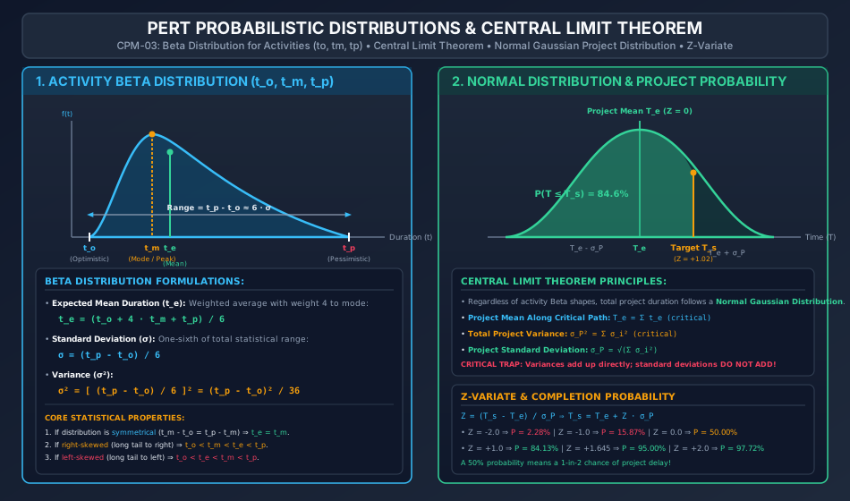
- Uncertainty is captured via Three-Time Estimates: Optimistic Time (), Most Likely Time (), and Pessimistic Time ().
- By virtue of the Central Limit Theorem, the sum of independent activity durations along any path approaches a Normal (Gaussian) Distribution, enabling rigorous statistical calculation of project completion probability for any contractual deadline ().
This master module presents an exhaustive treatment of PERT theory, mathematical derivations, network scheduling, probability density integration, and advanced network phenomena:
- Statistical Foundations: Mathematical derivation of expected activity duration () and activity variance () from the continuous Beta distribution.
- Network Scheduling: Forward and backward passes utilizing expected durations to isolate critical paths and calculate event slack.
- Central Limit Theorem & Normal Approximations: Aggregation of variances along the critical path () and formulating the standard normal variate ().
- The Variance Additivity Axiom: Proving why variances add algebraically along independent serial activities, whereas standard deviations do not add ().
- Merge Event Bias: Analytical deconstruction of classical PERT's systematic over-optimism at network convergence nodes, where multiple near-critical paths reduce true project completion probability.
2. Learning Objectives & Exam Weightage Analysis
Learning Objectives
- Contrast the core axioms of PERT (probabilistic, event-oriented, R&D focused) with CPM (deterministic, activity-oriented, construction focused).
- Define the three time estimates: Optimistic (), Most Likely (), and Pessimistic (), and explain why modal time is weighted fourfold in expected time derivations.
- Calculate activity expected duration () and variance () under the standard unimodal Beta distribution assumption.
- Execute network forward and backward passes using activity expected durations to establish the project expected completion time ().
- Compute the standard deviation () and variance () of the critical path using the variance additivity axiom.
- Calculate the probability of completing a project on or before an imposed contractual deadline () using the standard normal distribution table (-table).
- Determine the scheduled completion time required to achieve a specified confidence level (e.g., 50%, 84.1%, 90%, 95%, 99%).
- Analyze the phenomenon of Merge Event Bias and quantify the discrepancy between classical single-path PERT probability and true joint network probability.
Exam Weightage Analysis
| Exam Stream | Typical Question Type | Average Weightage | Recurring Focus Concepts |
|---|---|---|---|
| GATE CE | Numerical Answer Type (NAT) & MCQ | 2 – 4 Marks | Formulas for and ; calculating -index and project completion probability; critical path variance; identifying governing path when variances differ. |
| UPSC ESE (Prelims & Mains) | Objective + Multi-step Conventional | 10 – 20 Marks | Derivation of PERT Beta formulas; complete network evaluation with multiple paths; computing probability for various contractual dates ; merge event bias discussion. |
| SSC JE / RRB JE | Direct Objective Questions | 2 – 4 Questions | Formula for expected time (), standard deviation (), distribution type for activity (Beta) vs project (Normal). |
| State PSC AE/JE | Objective & Short Problem | 3 – 6 Marks | Differentiating PERT and CPM; calculation of and ; finding probability corresponding to , , and . |
3. Probabilistic Foundations: PERT vs CPM Philosophy & Event Orientation
3.1 Structural Comparison Between PERT and CPM
The fundamental distinctions between PERT and CPM govern their mathematical formulation and practical application in civil engineering:
+---------------------------------------------------------------------------------------------------+
| ATTRIBUTE           | PERT (Program Evaluation & Review)       | CPM (Critical Path Method)               |
+---------------------+------------------------------------------+------------------------------------------+
| Nature of Time      | Probabilistic (Three time estimates)     | Deterministic (Single time estimate)     |
| Orientation         | Event-Oriented (Milestones, States)      | Activity-Oriented (Work tasks, Ops)      |
| Project Domain      | Research & Development, Prototype Infr.  | Repetitive Construction, Maintenance     |
| Cost Considerations | Time-centric (Cost is secondary)         | Direct Cost-Time Trade-off (Crashing)    |
| Activity Distr.     | Beta Distribution (Continuous, Skewed)   | Constant / Uniform Point Estimate        |
| Project Distr.      | Normal Distribution (CLT Asymptotic)     | Deterministic Point Estimate             |
| Governing Metric    | Probability of Completion within Ts      | Critical Float ($TF = 0$) & Total Cost   |
+---------------------+------------------------------------------+------------------------------------------+
3.2 Event-Oriented Logic in PERT
While CPM emphasizes the execution of activities (consuming labor, plant, materials), PERT centers upon Events—instantaneous milestone points in time marking the start or completion of specific work phases.
- An event consumes neither time nor resources.
- Events are designated by nodes, and arrow lines denote precedence requirements.
- The temporal metric evaluated at each node is the Earliest Expected Event Time () and Latest Allowable Event Time ().
4. The Three-Time Estimates & The Beta Distribution Model
In novel infrastructure projects (e.g., deep sea tunneling, unmapped geological excavations, bespoke mega-bridges), activity durations cannot be stated deterministically. PERT models duration uncertainty using three subjective estimates obtained from experienced construction engineers.
       Probability
        Density
          f(t) ^                 Beta Distribution f(t)
               |                         *
               |                       *   *  Mode = tm
               |                     *       *
               |                   *           *
               |                 *               *
               |               *      Mean = te    *
               |             *            |          *
               |           *              |            *
               |       *                  |              *
               +-----+--------------------+---------------+-----> Duration (t)
                    to                   te              tp
              (Optimistic)            (Expected)    (Pessimistic)
4.1 The Three Estimates Defined
- Optimistic Time (): The minimum possible time required to complete the activity under ideal, extraordinarily favorable conditions where everything proceeds perfectly with zero unforeseen delays. The probability of completing faster than is statistically negligible ().
- Most Likely Time (): The modal duration representing the highest probability density in the frequency distribution. It is the duration that would occur most frequently if the activity were repeated numerous times under normal conditions.
- Pessimistic Time (): The maximum possible time required to complete the activity under extremely adverse, unfavorable circumstances (severe weather, labor walkouts, major material delivery failures). It does not, however, account for catastrophic "Acts of God" (war, earthquakes). The probability of exceeding is statistically negligible ().
The three estimates satisfy the strict order relation:
4.2 Analytical Derivation of Expected Time () and Variance ()
The probability density function of a standard continuous Beta distribution defined on the interval is:
In classical PERT formulation, two fundamental approximations are established:
-
Range Equal to Six Standard Deviations: Because and represent the lower and upper confidence boundaries (analogous to in a Gaussian model), the total practical range of the distribution encompasses standard deviations:
Consequently, the Activity Variance () is:
-
Weighted Mean Formulation: The expected value (mean duration ) is evaluated by approximating the continuous integral with a weighted cubic polynomial where the modal value () is given a weight of relative to the extreme bounds (Simpson's One-Third Rule weighting):
Skewness Characteristics of the Beta Distribution:
- Symmetric Distribution: When , the mode lies midway between the bounds. In this case, .
- Positively Skewed (Skewed Right): When , the mode is skewed toward , and the long tail extends toward . Here, . (Most common in civil construction).
- Negatively Skewed (Skewed Left): When , the mode is skewed toward , and the long tail extends toward . Here, .
5. Forward & Backward Pass on Expected Times (, Slack)
Once expected durations () are calculated for all network activities, the network is solved using standard CPM-style forward and backward recursive algorithms:
5.1 Earliest Expected Event Time ()
Moving from the project start node to the terminal node:
- Start Node: .
- Any Event :
5.2 Latest Allowable Event Time ()
Moving from the project terminal node back to the start node:
- Terminal Node: (unless an explicit contractual target is specified, in which case ).
- Any Event :
5.3 Event Slack ()
The slack of event is:
Events where (or minimum slack in the case of fixed targets) constitute the Critical Events, and the connected sequence of critical events forms the Critical Path.
6. Central Limit Theorem in Project Networks & Normal Distribution of Project Completion Time
While individual activity durations follow a skewed Beta Distribution, the total project duration along any path is the linear summation of multiple independent activity durations:
6.1 Statement of the Central Limit Theorem (CLT)
According to the Central Limit Theorem, the sum of a sufficiently large number () of independent random variables, each having finite mean and variance, converges asymptotically to a Normal (Gaussian) Distribution, regardless of the underlying probability distributions of the individual variables.
Therefore, the total duration of the critical path follows a Normal Distribution:
where:
- Project Expected Duration (): Sum of the expected times of all activities on the critical path:
- Project Variance (): Sum of the variances of all activities on the critical path:
- Project Standard Deviation ():
[!IMPORTANT] The Variance Additivity Axiom:
Variances are strictly additive for statistically independent activities: .
Standard deviations do NOT add!Computing by summing individual standard deviations and squaring will drastically overestimate project risk and is a fatal numerical error in competitive examinations!
7. Standard Normal Variate () & Project Completion Probability Computations
7.1 Formulation of the -Index
To determine the probability that the project will be completed on or before a specified scheduled contractual target time (), the normal distribution is normalized to the Standard Normal Distribution via the transformation:
where:
- Imposed scheduled completion target (contractual deadline).
- Expected critical path duration ().
- Critical path standard deviation ().
- Standard normal variate (number of standard deviations that deviates from ).
7.2 Probability Interpretation
The cumulative probability corresponds to the area under the standard normal curve from to :
+---------------------------------------------------------------------------------------------------+
| Z-VALUE   | PHYSICAL MEANING                                    | PROBABILITY P(Tp <= Ts)         |
+-----------+-----------------------------------------------------+---------------------------------+
| Z < 0     | Target Ts is BEFORE expected date Te (Ts < Te)       | P < 50.00%                      |
| Z = 0     | Target Ts EQUALS expected date Te (Ts = Te)          | P = 50.00%                      |
| Z > 0     | Target Ts is AFTER expected date Te (Ts > Te)        | P > 50.00%                      |
+---------------------------------------------------------------------------------------------------+
7.3 Standard -Score Conversion Table for Civil Examinations
The following exact cumulative normal distribution values are essential for rapid hand computation in GATE and ESE:
| -Score | Exam Engineering Context | |
|---|---|---|
| () | Extreme project delay () | |
| () | probability lower bound | |
| () | Lower envelope | |
| () | risk of meeting schedule | |
| () | Lower milestone () | |
| () | confidence benchmark | |
| () | Expected Baseline () | |
| () | contractor confidence level | |
| () | Upper milestone () | |
| () | commercial contractual threshold | |
| () | Standard 95% Confidence Interval () | |
| () | Upper envelope | |
| () | near-certainty engineering commitment | |
| () | Six-sigma upper bound () |
8. Critical Path Variance: The Variance Additivity Axiom
A critical property governing PERT network statistics is that only activities lying along the critical path contribute to the project variance . Non-critical activities, possessing positive float, can fluctuate within their float boundaries without altering the total project duration.
8.1 Competing Paths with Identical Mean Duration
When two or more network paths share the same maximum expected duration (), both paths are critical. However, their standard deviations may differ:
- Path 1:
- Path 2:
Which path governs project risk?
- If the target date is accelerated ():
The path with the larger variance gives a less negative , yielding a higher probability of completion! - If the target date is relaxed ():
The path with the smaller variance yields a higher , providing a much higher probability of completion!
Therefore, in networks with multiple critical paths, project completion probability must be evaluated along each path individually.
9. Sub-Critical Path Risk & The Merge Event Bias
9.1 The Fundamental Flaw of Classical PERT
Classical PERT computes project completion probability based exclusively on the single critical path, assuming that all sub-critical paths will finish on time and have zero influence on the project deadline.
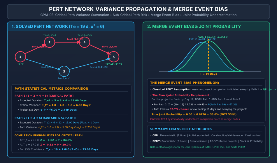
In reality, an event where multiple paths converge is a Merge Event. The project cannot finish until ALL converging paths have finished:
9.2 Mathematical Formulation of Merge Event Bias
Let Path 1 be the critical path (, ) and Path 2 be a near-critical sub-critical path (, ).
If both paths terminate at merge event , the project is completed on or before target if and only if both paths finish on or before :
Assuming statistical independence between the paths:
Quantitative Consequence:
For target (the expected duration of Path 1):
- Classical PERT evaluates only Path 1:
- Sub-critical Path 2 has:
- The true joint probability is:
[!CAUTION] Classical PERT reports a probability of on-time completion, whereas the true probability is only !
This discrepancy of over percentage points is known as the Merge Event Bias. In complex networks with many converging parallel paths, classical PERT drastically overestimates the likelihood of meeting project deadlines.
10. Contractual Target Dates, Penalty Horizons & Confidence Scheduling
In commercial infrastructure contracts, project tenders specify strict contractual completion horizons accompanied by severe financial liquidated damages for non-performance.
10.1 Confidence Interval Scheduling Equation
To guarantee a specific probability of on-time delivery (), the project manager must calculate the required scheduled duration () by rearranging the -variate equation:
+---------------------------------------------------------------------------------------------------+
| TARGET CONFIDENCE LEVEL | REQUIRED Z-SCORE | SCHEDULE EQUATION (TARGET BUFFER)                    |
+-------------------------+------------------+------------------------------------------------------+
| 50.0% (Base Mean)       | Z = 0.000        | Ts = Te                                              |
| 84.1% (One Sigma)       | Z = +1.000       | Ts = Te + 1.000 * sigma_P                            |
| 90.0% (Contract Target) | Z = +1.282       | Ts = Te + 1.282 * sigma_P                            |
| 95.0% (Industry Standard| Z = +1.645       | Ts = Te + 1.645 * sigma_P                            |
| 99.0% (Near Certainty)  | Z = +2.326       | Ts = Te + 2.326 * sigma_P                            |
+-------------------------+------------------+------------------------------------------------------+
The temporal difference represents the Statistical Contingency Buffer that must be incorporated into contractual bids to shield the contractor from liquidated damages.
11. Step-by-Step Rigorous Worked Numerical Examples
Problem 1: Complete PERT Network Reduction, Beta Statistics & Critical Path
Problem Statement:
A municipal water treatment facility project network consists of 5 events and 5 activities across two parallel paths converging at terminal event 5:
- Path 1: Activity
- Path 2: Activity
The three time estimates (in days) recorded by senior project engineers are:
- Activity :
- Activity :
- Activity :
- Activity :
- Activity :
Calculate:
- Expected duration () and variance () for every individual activity.
- The total expected duration and variance for both paths.
- Identify the Critical Path and determine the project expected completion time () and standard deviation ().
Step 1: Compute Expected Duration () and Variance () for Each Activity
Using and :
-
Activity :
-
Activity :
-
Activity :
-
Activity :
-
Activity :
Step 2: Summary of Activity Statistics
| Activity | (days) | (days) | (days) | |||
|---|---|---|---|---|---|---|
Step 3: Path Durations, Variances, and Critical Path Isolation
-
Path 1 ():
-
Path 2 ():
Since :
Problem 2: Project Completion Probability Analysis for Imposed Targets
Problem Statement:
For the water treatment facility analyzed in Problem 1 (, ):
- Compute the probability of completing the project on or before .
- Compute the probability of completing the project on or before an accelerated deadline .
- Determine the contractual completion time () the contractor must commit to in order to ensure a probability of finishing on schedule ().
Step 1: Probability for
Compute the standard normal variate :
From standard normal distribution tables:
(There is an probability of completing within days).
Step 2: Probability for
Compute the standard normal variate :
Using the symmetry property :
(There is only a chance of achieving the accelerated -day deadline).
Step 3: Scheduled Target for Confidence Level
For cumulative probability , the corresponding standard normal variate is:
Using the confidence scheduling equation:
Problem 3: Quantitative Proof of Merge Event Bias
Problem Statement:
In the network of Problem 1, both Path 1 () and Path 2 () terminate at event 5.
- Compute the classical PERT probability of completing the project by Day 19.0.
- Compute the individual probability that sub-critical Path 2 completes on or before Day 19.0.
- Assuming statistical independence, compute the true joint probability that the overall project completes on or before Day 19.0.
- Calculate the percentage point error introduced by classical PERT's omission of the sub-critical path.
Step 1: Classical PERT Probability
Classical PERT considers only the critical path (Path 1):
Step 2: Probability That Sub-Critical Path 2 Finishes by Day 19.0
For Path 2 ():
From the standard normal table:
Notice that there is a probability that sub-critical Path 2 will exceed 19 days!
Step 3: True Joint Project Completion Probability
The project terminates at event 5 only when both incoming paths have concluded:
Assuming statistical independence between the activities of Path 1 and Path 2:
Step 4: Quantifying the Merge Event Bias Error
Conclusion: Classical PERT overestimates the on-time project completion probability by over percentage points because it ignores the risk of the sub-critical path breaching the target date!
12. Comprehensive Exam Question Bank
Section A: GATE CE Previous Years & Anticipated Styles
-
[GATE CE NAT] An activity has optimistic, most likely, and pessimistic time estimates of 4, 7, and 16 days, respectively. The expected duration and standard deviation (in days) are, respectively:
- (A) 7.0 and 2.0
- (B) 8.0 and 2.0
- (C) 8.0 and 4.0
- (D) 9.0 and 2.0
Answer: (B). . .
-
[GATE CE NAT] A project has an expected duration of 40 days with a critical path standard deviation of 5 days. What is the probability that the project will be completed in 45 days? (Given )
Answer: .
Solution: . From standard normal table, . -
[GATE CE MCQ] In a PERT network, the critical path consists of three activities , and with standard deviations of 3, 4, and 5 days, respectively. The standard deviation of the project duration is:
- (A) 12.0 days
- (B) 7.07 days
- (C) 50.0 days
- (D) 4.0 days
Answer: (B). Variances add: . Project standard deviation is . (Notice: is the classic distractor!).
Section B: UPSC ESE Conventional Practice
- [ESE Mains] (a) State the basic assumptions underlying the PERT model.
(b) Explain why activity durations are assumed to follow a Beta distribution, whereas project duration follows a Normal distribution.
(c) A project critical path comprises five independent activities with variances and . The expected completion time is 60 days. Determine the contractual completion time that guarantees a probability of completion without penalty. ().
Solution Outline for (c): .
(or ).
Section C: SSC JE & State AE/JE Quick Fire
-
The frequency distribution of an activity in PERT analysis is assumed to be:
- (A) Normal distribution
- (B) Poisson distribution
- (C) Beta distribution
- (D) Exponential distribution
Answer: (C) Beta distribution.
-
The probability of completing a project within its expected time () is:
- (A)
- (B)
- (C)
- (D)
Answer: (B) (since ).
-
If the optimistic time is 3 days, most likely time is 6 days, and pessimistic time is 9 days, the variance of the activity is:
- (A) 1.0
- (B) 2.0
- (C) 6.0
- (D) 36.0
Answer: (A) .
-
In a PERT network, the critical path is defined as the path having:
- (A) Maximum variance
- (B) Minimum expected duration
- (C) Maximum expected duration
- (D) Minimum variance
Answer: (C) Maximum expected duration.
13. Common Conceptual Pitfalls & Field Traps
- Adding Standard Deviations Instead of Variances:
The most prevalent error in competitive exams is adding standard deviations directly (). Standard deviations are never additive; one must square to get variances, sum the variances (), and take the square root (). - Confusing Activity Distribution with Project Distribution:
Individual activity times follow the Beta Distribution (skewed, bounded between and ). The total project completion time follows the Normal Distribution by virtue of the Central Limit Theorem. - Pessimistic Time Exaggeration:
Mistaking for catastrophic disaster time (e.g., project destroyed by tsunami). assumes only normal adverse conditions within standard engineering parameters. - Ignoring Merge Event Bias:
Assuming that an on-time project delivery probability of on the critical path implies a overall project success rate. When near-critical paths merge, the actual project probability drops significantly below . - Negative -Score Calculation Trap:
When contractual target , is negative (). Students often drop the negative sign or look up directly, reporting probability instead of . Remember .
14. Quick Reference Formulas & Multi-Code Summary Table
| Category | Parameter | Exact Analytical Formulation |
|---|---|---|
| Activity Time Estimates | Expected Activity Duration () | |
| Activity Standard Deviation () | ||
| Activity Variance () | ||
| Network Scheduling | Earliest Event Time () | |
| Latest Event Time () | ||
| Event Slack () | ||
| Project Statistics | Project Expected Duration () | |
| Project Variance () | ||
| Project Standard Deviation () | ||
| Probability Index | Standard Normal Variate () | |
| Scheduled Completion Target () | ||
| Merge Event Probability | Independent Joint Probability | |
| Key Confidence Levels | Probability | |
| Probability | ||
| Probability | ||
| Probability |