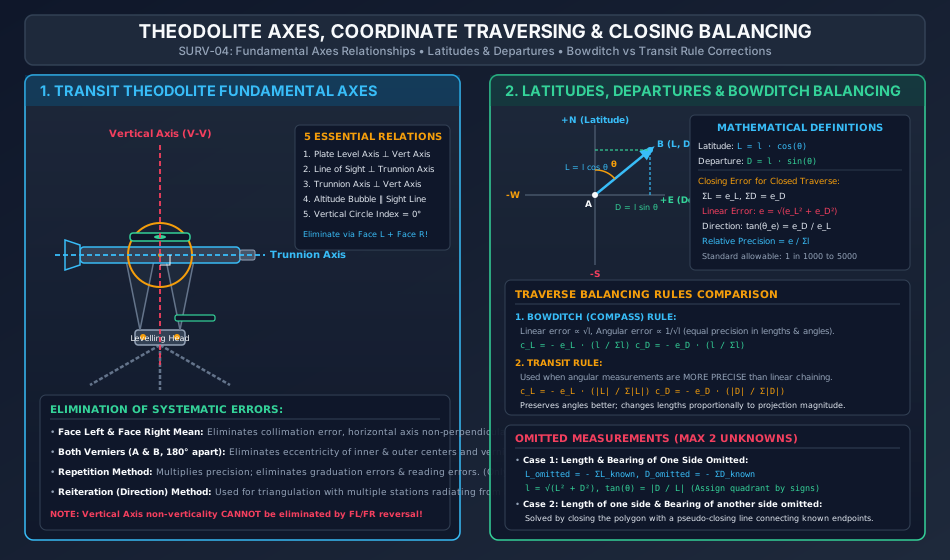
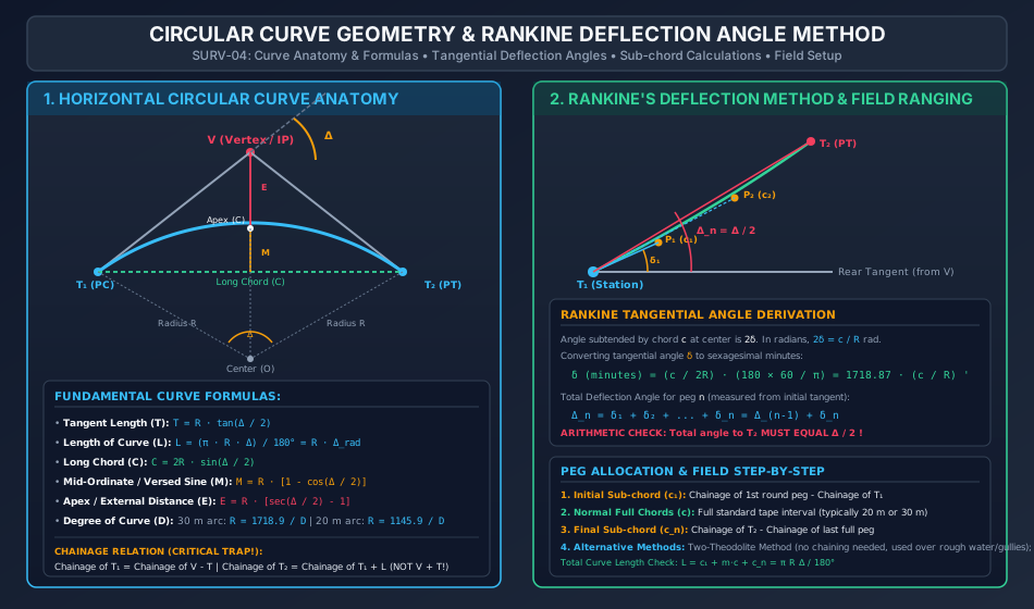
The transit theodolite is the premier optical-mechanical instrument of engineering geomatics, serving as the universal standard for precise angular measurement in both horizontal and vertical planes. In civil engineering infrastructure—spanning highways, railways, tunneling, dams, pipelines, and cadastral boundary demarcations—theodolite traversing provides the rigid geometric skeleton upon which all secondary topographic details and construction alignments depend.
This comprehensive master module synthesizes:
Instrumental Mechanics & Geometry: Fundamental axes of the transit theodolite, geometric relationships, temporary and permanent adjustments, and the elimination of systematic instrumental collimation, trunnion axis tilt, and index errors via Face Left/Face Right observations.
Coordinate Geometry of Traverses: Computation of Latitudes (L=lcosθ) and Departures (D=lsinθ), conversion between consecutive (dependent) coordinates and total (independent) coordinates (Gale's Traverse Table), closing error vectors (e=ΣL2+ΣD2), and rigorous traverse balancing methods (Bowditch Compass Rule, Transit Rule, and Axis Rule).
Missing / Omitted Measurements: Mathematical resolution of up to two unknown geometric quantities (lengths or bearings) utilizing closed polygon vector conditions (ΣL=0, ΣD=0).
Horizontal Circular Curve Ranging: Geometry of simple circular curves, tangent distances, curve lengths, long chords, mid-ordinates (versed sine), apex distances, chainage continuity, and setting out via linear chord methods, two-theodolite intersections, and Rankine's Tangential Deflection Angle Method with sub-chord allocation.
2. Learning Objectives & Exam Weightage Analysis
Learning Objectives
State and derive the 5 fundamental axes relationships of a transit theodolite and explain why Face Left and Face Right reversal eliminates horizontal collimation error, trunnion axis tilt, and vertical circle index error, but cannot eliminate plate vertical axis tilt.
Calculate consecutive coordinates (Latitude and Departure) from whole circle bearings and slope-corrected horizontal lengths.
Quantify traverse closing error (e), relative precision (e/Σl), and apply Bowditch's Rule and Transit Rule corrections with mathematical justification.
Solve missing traverse measurements involving one side completely omitted or two sides with one missing parameter each.
Derive simple circular curve geometric formulas from fundamental circle theorems and establish correct station chainages.
Calculate tangential deflection angles (δi=1718.87ci/R min) and construct a complete field ranging table for Rankine's method.
Rankine's deflection formula (1718.87c/R), Chainage of PC/PT, closing error vector direction.
3. Theodolite Anatomy, Fundamental Axes & Instrumental Geometry
A transit theodolite is characterized by its telescope being capable of a complete 360∘ rotation about its horizontal (trunnion) axis in the vertical plane.
3.1 Fundamental Lines and Axes
Vertical Axis (V−V): The axis about which the instrument rotates in the horizontal plane (axis of the inner and outer centers).
Horizontal Axis / Trunnion Axis (H−H): The axis about which the telescope rotates in the vertical plane.
Line of Collimation (Line of Sight): The imaginary line passing through the optical center of the objective lens and the intersection of the cross-hairs of the reticle.
Axis of the Plate Level: The straight line tangential to the internal longitudinal curve of the plate bubble tube at its center point.
Axis of the Altitude Bubble Tube: The line tangential to the longitudinal curvature of the telescope or index level tube at its center.
3.2 Five Desired Geometric Relationships
In an ideally adjusted theodolite:
Plate Level Axis ⊥ Vertical Axis: Ensures the horizontal plate is truly horizontal when the plate bubble is centered.
Line of Sight ⊥ Horizontal (Trunnion) Axis: Ensures the line of collimation traces a true plane (not a cone) when plunged.
Horizontal (Trunnion) Axis ⊥ Vertical Axis: Ensures the line of collimation rotates in a truly vertical plane.
Altitude Bubble Axis ∥ Line of Sight: Ensures true zero vertical datum when the telescope is horizontal.
Vertical Circle Vernier reads 0∘00′00′′ when line of sight is horizontal.
Produces horizontal angular displacement β=c⋅secα (where α is elevation angle).
Take mean of Face Left (Circle Left) and Face Right (Circle Right) observations.
YES
Trunnion Axis not ⊥ Vertical Axis
Produces horizontal pointing error i=b⋅tanα. Significant on steep sights.
Take mean of Face Left and Face Right observations.
YES
Vertical Circle Index Error
Systematic offset on vertical angles (αobs=αtrue±ϵ).
Take mean of Face Left and Face Right vertical angles: α=2αL+αR.
YES
Eccentricity of Inner & Outer Centers
Reading offset variable across graduated circle.
Read both Verniers (A and B) positioned 180∘ apart and average them.
YES (via Dual Verniers)
Eccentricity of Verniers
Zero of verniers not exactly 180∘ opposite.
Read both Verniers (A and B) and take mean.
YES (via Dual Verniers)
Non-Verticality of Vertical Axis
Causes trunnion axis and line of sight to trace oblique paths; error varies dynamically with azimuthal direction.
CANNOT BE ELIMINATED BY FACE REVERSAL! Must be corrected strictly by careful levelling using plate foot screws.
NO (Fatal Error!)
4.1 Horizontal Angle Measurement Techniques
Repetition Method: Angle measured multiple times (n times) consecutively along the circle without resetting. Final reading divided by n.
θ=nFinal Reading+m⋅360∘−Initial ReadingEliminates graduation errors and reading errors; applicable ONLY to horizontal angles.
Reiteration (Direction) Method: Several angles measured from a single central instrument station to multiple surrounding stations by sighting in sequence and "closing the horizon" back to the reference station. Preferred in primary triangulation.
A traverse consists of a connected sequence of survey lines whose lengths are measured linearly (chain/tape/EDM) and whose relative directions are measured angularly (theodolite/compass).
5.1 Latitudes and Departures
For a traverse line AB having length l and Whole Circle Bearing θ:
Latitude (L): Orthographic projection on the reference North-South meridian.
L=lcosθ
If pointing North (0∘≤θ<90∘ or 270∘<θ≤360∘): Latitude is Positive (Northing).
If pointing South (90∘<θ<270∘): Latitude is Negative (Southing).
Departure (D): Orthographic projection on the reference East-West line.
D=lsinθ
If pointing East (0∘<θ<180∘): Departure is Positive (Easting).
If pointing West (180∘<θ<360∘): Departure is Negative (Westing).
       Quadrant I (NE)  :  L = + l cos θ,  D = + l sin θ
       Quadrant II (SE) :  L = - l cos θ,  D = + l sin θ
       Quadrant III (SW):  L = - l cos θ,  D = - l sin θ
       Quadrant IV (NW) :  L = + l cos θ,  D = - l sin θ
5.2 Closing Error of a Closed Traverse
In a mathematically perfect closed loop traverse returning to its origin:
∑L=0and∑D=0
Due to random observational errors, practical surveys yield non-zero closures:
∑L=eL(Error in Latitude),∑D=eD(Error in Departure)
Magnitude of Total Linear Closing Error (e):e=eL2+eD2
Direction (Bearing) of Closing Error (θe):tanθe=eLeD⟹θe=arctan(∣eL∣∣eD∣)(Assigned to proper quadrant based on signs of eL and eD).
Relative Precision (Degree of Accuracy):Relative Precision=∑le=(e∑l)1(Expressed as 1 in N; standard cadastral requires 1:1000 to 1:3000, geodetic control >1:10000).
6. Traverse Balancing Mathematical Rules
When the closing error falls within permissible tolerances, it must be distributed across the traverse lines to close the mathematical polygon.
+---------------------------------------------------------------------------------------------------+
| METHOD              | CORRECTION TO LATITUDE (c_L)           | CORRECTION TO DEPARTURE (c_D)          |
+---------------------+----------------------------------------+----------------------------------------+
| Bowditch's Rule     | c_L = - e_L * ( l / \Sigma l )         | c_D = - e_D * ( l / \Sigma l )         |
| (Compass Rule)      |                                        |                                        |
+---------------------+----------------------------------------+----------------------------------------+
| Transit Rule        | c_L = - e_L * ( |L| / \Sigma |L| )     | c_D = - e_D * ( |D| / \Sigma |D| )     |
+---------------------+----------------------------------------+----------------------------------------+
| Axis Rule           | Line lengths held fixed; corrections applied purely to line directions.         |
+---------------------+----------------------------------------+----------------------------------------+
6.1 Bowditch's (Compass) Rule
Foundational Assumptions:
Linear measurements are made with chain/tape where errors are accidental: Elinear∝l.
Angular measurements are made with compass/theodolite where errors are accidental: Eangular∝l1.
Total error distribution weights lengths and angles equally.
When physical obstructions (rivers, dense structures, steep ravines) prevent direct measurement of a line, missing values are deduced mathematically because a closed polygon provides two independent scalar equilibrium equations:
For 30 m Arc Definition:R=πD30×180∘≈D1718.87≈D1719 m
For 20 m Arc Definition:R=πD20×180∘≈D1145.92≈D1146 m
8.3 Chainage Calculation Sequence (Critical Rule)
Curve chainage follows the actual path of travel along the curve arc:
Chainage of PC (T1)=Chainage of Vertex (V)−TChainage of PT (T2)=Chainage of PC (T1)+LChainage of T2=Chainage of V+T(Common Trapping Error!)
9. Linear & Angular Methods of Curve Ranging
9.1 Linear Methods (Chain and Tape Only)
Used when high optical precision is not required or instruments are unavailable:
Offsets from Long Chord:Ox=R2−x2−(R−M)≈M−2Rx2(where x is distance measured from midpoint of long chord).
Offsets from Tangents:
Radial offsets: Ox=R2+x2−R≈2Rx2
Perpendicular offsets: Ox=R−R2−x2≈2Rx2
Offsets from Chords Produced:
First chord offset: O1=2Rc12
Intermediate chords: Oi=2Rc(c+ci−1); for equal chords c: O=Rc2
Last chord offset: On=2Rcn(c+cn)
9.2 Angular Methods (Theodolite Based)
Rankine's Tangential Deflection Angle Method: Single theodolite at T1, tape for chord measurements. Standard highway/railway technique.
Two-Theodolite Method: Instruments placed at both T1 and T2. No linear taping needed; points located by optical intersection of simultaneous sightlines (Δi from T1 and Δ−Δi from T2). Ideal for steep ravines, swift rivers, and rough ground.
10. Rankine's Method of Tangential Angles & Detailed Deflection Computations
10.1 Mathematical Derivation
Let P1,P2,…,Pn be points pegged on the curve arc at chord lengths c1,c2,…,cn.
The angle subtended by chord ci at the center of the curve is 2δi.
By the geometric property of a circle, the tangential angle δi between the tangent at the chord start and the chord itself is half the central angle:
Central angle=2δi=Rci radians⟹δi=2Rci radians
Converting radians to sexagesimal minutes:
δi=2Rci×π180∘×60′=2Rci×π10800′=π5400⋅Rci=1718.873⋅Rci minutesδi(minutes)=1718.87×Rci(ci,R in meters)
10.2 Total Deflection Angles (Δi)
The total deflection angle Δi measured from the initial tangent VT1 to station Pi is the cumulative sum of all preceding tangential angles:
Problem 2: Resolution of Omitted Traverse Measurements
Problem Statement:
In the 4-sided closed traverse ABCD, boundary obstructions prevented the measurement of both the length and bearing of line DA. The remaining survey measurements are:
Line AB: l=100.00 m, Bearing =30∘00′
Line BC: l=150.00 m, Bearing =110∘00′
Line CD: l=120.00 m, Bearing =210∘00′
Determine the length and whole circle bearing of line DA.
Step 1: Compute Latitudes and Departures of Known Lines
From Problem 1:
Line AB: L=+86.603 m, D=+50.000 m
Line BC: L=−51.303 m, D=+140.954 m
Line CD: L=−103.923 m, D=−60.000 m
Step 2: Sum Known Coordinates
∑Lknown=+86.603−51.303−103.923=−68.623 m∑Dknown=+50.000+140.954−60.000=+130.954 m
Step 3: Apply Equilibrium Conditions for Line DA
∑L=0⟹∑Lknown+LDA=0⟹LDA=−∑Lknown=−(−68.623)=+68.623 m∑D=0⟹∑Dknown+DDA=0⟹DDA=−∑Dknown=−(+130.954)=−130.954 m
Problem 3: Setting Out a Circular Curve by Rankine's Method
Problem Statement:
Two straights intersect at chainage 2450.00 m with a deflection angle Δ=48∘00′. A simple circular curve of radius R=300.00 m is to be set out using a transit theodolite and standard peg interval of 20.00 m.
Calculate:
Tangent length, curve length, and chainages of PC (T1) and PT (T2).
Length of the initial sub-chord, number of standard chords, and length of the final sub-chord.
Individual tangential angles (δi) and total deflection angles (Δi) for setting out all pegs.
Step 1: Curve Parameters
Tangent Length (T):T=Rtan(2Δ)=300.00×tan(24∘)=300.00×0.445229=133.569 m
Length of Curve (L):L=180∘πRΔ=180∘π×300.00×48∘=80π=251.327 m
Chainages:Chainage of PC (T1)=Chainage of V−T=2450.00−133.569=2316.431 mChainage of PT (T2)=Chainage of T1+L=2316.431+251.327=2567.758 m
Step 2: Chord Allocation
The standard peg interval is 20.00 m.
Chainage of T1=2316.431 m. The first whole peg on the curve is at chainage 2320.00 m.
c1=2320.00−2316.431=3.569 m(Initial sub-chord)
Full pegs run from 2320.00 m up to 2560.00 m:
nfull=20.002560.00−2320.00=12 full chords of 20.00 m
Chainage of last full peg =2560.00 m. Chainage of T2=2567.758 m:
cn=2567.758−2560.00=7.758 m(Final sub-chord)
Verification of total chord lengths:
∑c=3.569+(12×20.00)+7.758=3.569+240.00+7.758=251.327 m=L[Exact!]
Section A: GATE CE Previous Years & Anticipated Styles
[GATE CE] In a closed traverse ABCD, the sum of latitudes is −1.20 m and the sum of departures is +1.60 m. The perimeter of the traverse is 1000 m. If the length of line AB is 250 m, the Bowditch correction to the latitude of line AB is:
(A) +0.30 m
(B) −0.30 m
(C) +0.40 m
(D) −0.40 m Answer: (A). cL=−eL∑ll=−(−1.20)×1000250=+0.30 m.
[GATE CE] A circular curve of radius 400 m has a deflection angle of 60∘. If the chainage of the intersection point is 1500.00 m, the chainage of the point of curvature (PC) in meters is:
(A) 1269.06 m
(B) 1230.94 m
(C) 1080.97 m
(D) 1730.94 m Answer: (A). T=Rtan(Δ/2)=400×tan30∘=400×0.57735=230.94 m. Chainage =1500.00−230.94=1269.06 m.
Section B: UPSC ESE Conventional Practice
[ESE Mains] Explain with mathematical diagrams why the Bowditch rule is preferred when linear measurements are made with a chain and angles with a compass, whereas the Transit rule is preferred when theodolite angular observations are of superior precision. State the equations for both and show how relative weights are assigned.
Section C: SSC JE & State AE/JE Quick Fire
The method of measuring horizontal angles most suited for establishing control networks with multiple radiation lines from a single instrument hub is:
In Rankine's method of deflection angles, the tangential angle δ in minutes for a chord c and radius R is given by:
(A) 1718.87cR
(B) 1718.87Rc
(C) 57.3Rc
(D) 1146Rc Answer: (B).
Which of the following instrumental errors CANNOT be eliminated by taking the mean of Face Left and Face Right theodolite observations?
(A) Horizontal collimation error
(B) Index error of vertical circle
(C) Non-perpendicularity of trunnion axis to vertical axis
(D) Non-verticality of the vertical axis Answer: (D).
13. Common Conceptual Pitfalls & Field Traps
PT Chainage Addition Trap:
Calculating chainage of PT (T2) as Chainage of V+T. Field Reality: Vehicles travel along the curved arc T1T2, not along the straight tangents through V. Always compute:
Chainage of T2=Chainage of T1+L
Bowditch Sign Convention Trap:
Applying corrections with the same sign as the closing error. Field Reality: A negative closure (eL<0) indicates the polygon fell short; hence corrections must be positive (+) to expand the perimeter and close the gap:
Correction=−(Error)
Transit Rule Absolute Denominator Trap:
Using algebraic sums ∑L in the denominator of the Transit rule rather than the sum of absolute values ∑∣L∣. Field Reality: Algebraic sum ∑L is simply the error eL! The Transit rule denominator must be ∑∣L∣=∑(Northings)+∑(Southings).
Rankine Tangential vs Central Angle Trap:
Confusing the tangential deflection angle δ with the central angle subtended by the chord (2δ). The tangential angle is strictly half the central angle!
Level Bubble Sensitivity Trap:
Assuming face reversal cures plate bubble unlevelness. If the vertical axis is tilted by ϵ, it remains tilted by ϵ after a 180∘ rotation; the error cannot be eliminated optically and corrupts all horizontal pointing.