Water Demand Forecasting, Population Projection & Water Quality Parameters
In this chapter (1 topics)
On this page
- 1. Topic Title & Authoritative References
- 2. Prerequisites & Learning Objectives
- Prerequisites
- Learning Objectives
- 3. Water Demands, Variations & Fire Demand Formulations
- 3.1 Design Periods of Water Supply Infrastructure Components
- 3.2 Municipal Water Demand Breakdown per IS 1172:1993
- 3.3 Temporal Demand Variations & Peaking Factors
- 3.4 Fire Demand Formulations & The Coincident Draft
- 4. Population Forecasting Methodologies
- 4.1 Arithmetic Increase Method
- 4.2 Geometric Increase (Uniform Rate) Method
- 4.3 Incremental Increase Method
- 4.4 Decreasing Rate of Growth Method
- 4.5 The Logistic S-Curve (Verhulst Model)
- 5. Physical Water Quality Parameters & Analytical Methods
- 5.1 Turbidity
- 5.2 Color
- 5.3 Taste & Odor
- 5.4 Total Dissolved Solids (TDS) & Electrical Conductivity (EC)
- 6. Chemical Water Quality Parameters & Aquatic Stoichiometry
- 6.1 pH and Hydrogen Ion Activity
- 6.2 Alkalinity: Chemistry & Titration Endpoints
- 6.3 Total Hardness & Hardness Partitioning
- 6.4 Chlorides (Cl-)
- 6.5 Fluorides (F-)
- 6.6 Nitrogen Forms & Diagnostic Pollution Chronology
- 6.7 Toxic Metals & Heavy Contaminants
- 7. Biological Water Quality Parameters & Bacteriological Testing
- 7.1 Criteria for an Ideal Indicator Organism
- 7.2 The Coliform Group
- 7.3 Multiple Tube Fermentation Test (MTFT)
- 7.4 Most Probable Number (MPN) & Thomas Approximation
- 7.5 Membrane Filter (MF) Technique
- 8. Comparative Codal Standards Matrix: IS 10500:2012 vs WHO
- 9. Water Supply Engineering Design Periods & Component Capacities
- 10. Step-by-Step Analytical Derivations & Quantitative Formulations
- 10.1 Analytical Derivation of the Verhulst Logistic Growth Model
- 10.2 Stoichiometric Derivation of Water Hardness and Alkalinity
- 11. Solved Numerical Examples (Pre-Calculated & Python-Verified)
- Problem 1: Population Forecasting & Municipal Water Supply System Design
- Problem 2: Complete Ionic Water Analysis, Hardness & Alkalinity Partitioning
- Problem 3: Biological Water Quality Testing & MPN Coliform Quantification
- 12. Common Misconceptions, Pitfalls & Exam Traps
- 13. Practice Problems (Curated for Competitive Examinations)
- Level 1: Objective & Conceptual (SSC JE / RRB JE / State AE)
- Level 2: Analytical & Multi-Step (GATE CE / UPSC ESE)
- 14. Quick Revision Summary & Memory Hooks
- Core Numerical Constants & Codal Rules
1. Topic Title & Authoritative References
Title: Municipal Water Demand Forecasting, Population Projection Mathematics, Diurnal Peaking Dynamics, Fire Flow Hydraulics, Comprehensive Physical-Chemical-Biological Water Quality Parameters, and Drinking Water Specifications (IS 10500:2012).
Primary Standards & Authoritative Specifications:
- IS 10500:2012: Drinking Water — Specification (Second Revision, with Amendments 1, 2 & 3).
- IS 1172:1993: Code of Basic Requirements for Water Supply, Drainage and Sanitation (Fourth Revision).
- CPHEEO Manual (1999 / 2024 draft): Manual on Water Supply and Treatment, Central Public Health and Environmental Engineering Organisation, Ministry of Housing and Urban Affairs (MoHUA), Government of India.
- WHO (2017 / 2022): Guidelines for Drinking-water Quality (Fourth Edition incorporating the First and Second Addenda).
- Standard Methods for the Examination of Water and Wastewater (APHA, AWWA, WEF, 23rd/24th Editions).
2. Prerequisites & Learning Objectives
Prerequisites
- Stoichiometric chemistry: gram equivalent weights, valence, normality (), molarity (), milliequivalents per liter (), and logarithmic scales ().
- Differential equations: first-order growth models, separable ordinary differential equations, and logistic saturation functions.
- Hydraulic fundamentals: volumetric discharge rate (), mass conservation, and pressure head ().
Learning Objectives
- Quantify municipal water demand categories per IS 1172 (domestic , commercial, industrial, public, fire flow, and unaccounted-for water / distribution losses).
- Formulate diurnal consumption curves, determine Goodrich peaking factors, and compute the critical Coincident Draft () for distribution mains.
- Derive and apply analytical population forecasting models: Arithmetic Increase, Geometric Increase ( geometric mean), Incremental Increase, Decreasing Rate of Growth, and the Verhulst Logistic S-Curve.
- Evaluate physical water quality parameters: Turbidity (Jackson candle extinction vs Nephelometric light scatter NTU), Color (Platinum-Cobalt Hazen units), Taste and Odor (Threshold Odor Number, ), and Total Dissolved Solids ().
- Master chemical aquatic stoichiometry: Phenolphthalein () and Total () alkalinity titration endpoints, Total Hardness (), and partitioning into Carbonate Hardness () and Non-Carbonate Hardness ().
- Analyze public health toxicology: Fluoride concentration thresholds ( caries vs dental fluorosis vs skeletal fluorosis), Nitrate reduction causing infant methemoglobinemia (Blue Baby Disease), and heavy metal toxicities (Arsenic, Lead, Cadmium, Mercury).
- Execute biological water testing: coliform indicator taxonomy, Multiple Tube Fermentation Test (MTFT: Presumptive, Confirmed, Completed), Thomas approximation formula for Most Probable Number (), Membrane Filtration (), and statutory zero-tolerance coliform standards.
3. Water Demands, Variations & Fire Demand Formulations
3.1 Design Periods of Water Supply Infrastructure Components
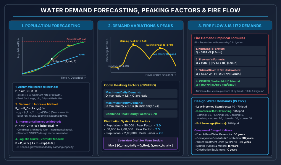
Water supply projects are designed for a prospective future horizon known as the Design Period. The design period balances capital cost economy, physical asset lifespan, ease of future expansion, and financial debt amortization:
| Infrastructure Component | Statutory Design Period (Years) | Limiting Design Criteria / Governing Factor |
|---|---|---|
| Storage Reservoirs & Dams | High capital expenditure; impractical to enlarge incrementally | |
| Raw Water Conveyance Conduits & Mains | Excavation, right-of-way, and pipe laying economies of scale | |
| Water Treatment Plant (WTP) Units | Modular expansion in parallel phases every years | |
| Electric High-Lift / Low-Lift Pumps | Mechanical wear, impeller cavitation, and rapid motor obsolescence | |
| Treated Water Distribution Pipe Network | Disruptive urban road excavation; designed for ultimate capacity | |
| Service Reservoirs (Overhead Tanks / ESR) | Balancing diurnal fluctuations and emergency fire storage | |
| Chlorinators & Chemical Dosing Feeders | Corrosive chemical degradation and technological upgrades |
3.2 Municipal Water Demand Breakdown per IS 1172:1993
- Domestic Water Consumption:
- Low-Income Group / Rural / Standpost Supply: (liters per capita per day).
- Communities with full flushing systems (Towns & Cities): (Standard design benchmark per IS 1172):
- Bathing:
- Toilet Flushing:
- Washing of clothes:
- Washing of utensils:
- House cleaning:
- Cooking:
- Drinking:
- Total Domestic: .
- Metropolitan Cities with Full Sewerage Systems: .
- Commercial & Institutional Demands: Schools (), hospitals (), hotels (), offices (). Typically accounts for average across municipality.
- Industrial Water Demand: Highly variable depending on industrial zoning ().
- Public Utility / Civic Uses: Street washing, public parks, sewer flushing, fountains (, approx of total).
- Unaccounted-for Water (UFW) & Distribution Losses: Leaking pipe joints, valve gland weepage, pipe bursts, unauthorized illegal connections, meter inaccuracies. CPHEEO mandates provision of of total municipal demand for distribution losses.
- Total Average Municipal Consumption:
3.3 Temporal Demand Variations & Peaking Factors
Water consumption fluctuates seasonally, daily, and hourly. The seasonal peak occurs in hot summer months; the weekly peak occurs on weekends; the diurnal variation exhibits two distinct peaks (morning domestic rush and evening cooking/bathing rush ), separated by a midday drop and a deep night trough ().
Goodrich Peaking Formulation
Goodrich (1931) formulated the empirical relationship between the duration of demand (days) and peak percentage of average annual demand:
- For (Maximum Daily Demand):
- For (Maximum Weekly Demand):
- For (Maximum Monthly Demand):
Hourly Peaking & Peak Factors per CPHEEO
The maximum hourly demand on the day of maximum consumption is:
For distribution network hydraulic design, CPHEEO specifies the Peak Factor () based on population size:
- Population :
- Population :
- Population :
3.4 Fire Demand Formulations & The Coincident Draft
Fire fighting requires immense flow rates for short durations ( continuous fire streams) at high pressure ( or head at fire hydrants).
Authoritative Empirical Fire Demand Formulas
Let be population in thousands ():
- Kuichling's Formula:
- Freeman's Formula:
- National Board of Fire Underwriters (NBFU) Formula:
- Buston's Formula:
- CPHEEO / Indian Ministry of Urban Development Formula:
The Coincident Draft Rule
A catastrophic municipal fire can erupt simultaneously with the maximum daily domestic consumption, but is statistically improbable to coincide exactly with the single highest peak hour. Therefore, municipal distribution mains must be proportioned for the Coincident Draft:
- Treatment plant units, raw water pumps, and supply conduits are designed for .
- Distribution pipelines are designed for the Coincident Draft.
- Service reservoirs (ESR) supply the balancing volume difference between variable hourly consumption and constant 24-hr pumping.
4. Population Forecasting Methodologies
Accurate estimation of the design population () after decades is essential for water supply sizing. Five classical methods are used depending on the city's age, growth trajectory, and geographic constraints:
4.1 Arithmetic Increase Method
- Hypothesis: Rate of population growth with respect to time is constant:
- Mathematical Formulation: where is latest known census population, is number of decades to forecast, and is arithmetic mean of historical decadal population increases:
- Field Applicability: Strictly suited for large, old, mature, highly congested cities that have reached near-saturation density with limited scope for horizontal suburban expansion. Yields conservative (lower bound) estimates.
4.2 Geometric Increase (Uniform Rate) Method
- Hypothesis: Rate of population growth is proportional to the existing population:
- Discrete Compounding Formulation: where is the geometric mean percentage growth rate across historical decades: or alternatively via logarithmic transformation:
- Field Applicability: Best suited for young, rapidly expanding cities, new industrial hubs, and economic growth corridors. Yields aggressive (upper bound) estimates; overestimates future population if applied to aging cities.
4.3 Incremental Increase Method
- Hypothesis: Modifies the constant arithmetic rate by superimposing an incremental acceleration or deceleration factor ():
where:
- is average decadal arithmetic increase.
- is average decadal incremental increase (increase over the previous increase).
- Field Applicability: Recommended by CPHEEO for standard municipal master plans. Strikes a rational balance between arithmetic conservatism and geometric compounding.
4.4 Decreasing Rate of Growth Method
- Hypothesis: As a city approaches its ultimate physical carrying capacity, the percentage growth rate () decreases systematically by an average decadal decrement ():
- Field Applicability: Cities with limited land availability, ring-fenced by natural barriers (mountains, oceans) or urban green belts.
4.5 The Logistic S-Curve (Verhulst Model)
Under unrestricted early conditions, population grows exponentially; as density approaches environmental carrying capacity (), growth is throttled by congestion, real estate costs, and resource scarcity:
Integrating with initial condition at :
- Point of Inflection: Occurs at , where the rate of growth reaches its mathematical maximum (). Before inflection, growth accelerates (); past inflection, growth decelerates asymptotically toward .
- Three-Point Calibration Formula (McLean): If census data is available at three equidistant time intervals ():
5. Physical Water Quality Parameters & Analytical Methods
Physical parameters originate from contact with soil strata, decaying vegetative matter, and colloidal suspensions:
5.1 Turbidity
- Definition & Environmental Physics: Turbidity is an optical property that causes light to be scattered and absorbed rather than transmitted in straight lines through a water sample. It is caused by suspended and colloidal matter such as clay, silt, finely divided organic and inorganic matter, and microscopic plankton.
- Interfering Impact: Shields pathogenic bacteria, viruses, and helminth cysts from contact with chemical disinfectants (chlorine, ozone, UV rays), shielding them against disinfection.
- Analytical Instruments:
- Jackson Candle Turbidimeter (JTU): Visual light extinction method. Water poured into a calibrated glass tube placed over a standard spermaceti candle flame until the flame image vanishes into uniform glow. Cannot measure turbidity ; obsolete for drinking water; used for raw flood waters.
- Nephelometer (Nephelometric Turbidity Units, NTU): Photoelectric detection of scattered light measured at a right angle to the incident light beam. Uses a tungsten filament lamp () and a photodiode detector.
- Standard Reference Suspension: Formazin polymer, formed by reacting equal volumes of hydrazine sulfate () and hexamethylenetetramine () in distilled water (produces stock).
- IS 10500:2012 Limits: Acceptable Limit ; Permissible Limit in absence of alternate source .
5.2 Color
- Source: True color is caused by dissolved vegetable extracts, humic acids, fulvic acids, peat, and mineral colloids (). Apparent color includes suspended matter turbidity.
- Measurement: Measured by visual comparison with calibrated standard glass color discs or platinum-cobalt solutions (Platinum-Cobalt Scale / Hazen Scale).
- Standard Unit (1 Hazen Unit): The color produced by dissolving of platinum (as potassium chloroplatinate, ) and of cobaltous chloride () in of distilled water.
- IS 10500:2012 Limits: Acceptable Limit ; Permissible Limit .
5.3 Taste & Odor
- Source: Volatile compounds produced by algae (Anabaena, Microcystis producing geosmin and 2-methylisoborneol), rotting aquatic vegetation, industrial phenols, and hydrogen sulfide ().
- Measurement (Threshold Odor Number, ): where is volume of odorous water sample (), and is volume of odor-free dilution distilled water () required to yield a mixture in which odor is just barely perceptible to a trained panel at .
- Flavor Threshold Number (): Analogous dilution ratio for taste.
- IS 10500:2012 Limits: Agreeable ( to ).
5.4 Total Dissolved Solids (TDS) & Electrical Conductivity (EC)
- Analytical Method: Gravimetric determination. Water sample filtered through a standard glass fiber filter (), and the filtrate is evaporated to dryness in a tared platinum or porcelain dish in an oven at until constant weight is attained. (Drying at drives off mechanically occluded water and decomposes bicarbonates to carbonates).
- Conductivity Relationship: Electrical conductivity () in at provides an instantaneous surrogate measurement for mineral ion content:
- IS 10500:2012 Limits: Acceptable Limit ; Permissible Limit .
6. Chemical Water Quality Parameters & Aquatic Stoichiometry
6.1 pH and Hydrogen Ion Activity
- Definition: Negative base-10 logarithm of hydrogen ion activity:
- Equilibrium at :
- Engineering Significance: Controls chemical coagulation efficiency (alum optimum pH ), chlorine speciation ( vs ), scale formation versus pipe corrosion.
- IS 10500:2012 Limits: (Strict limit; NO RELAXATION permitted).
6.2 Alkalinity: Chemistry & Titration Endpoints
Alkalinity is the quantitative capacity of aquatic species to neutralize hydrogen ions (). It acts as a chemical buffer against pH drops. In natural waters, alkalinity is imparted almost exclusively by three basic anions: Hydroxide (), Carbonate (), and Bicarbonate ().
Converting ionic concentrations from to equivalent :
where Equivalent Weight of .
Titration Kinetics & Endpoints
A water sample is titrated against standardized :
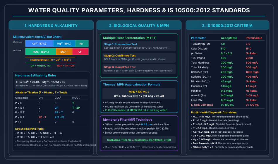
- Phenolphthalein Alkalinity (): Titrated until pink color discharges at pH . At pH , all is neutralized, and all is converted to :
- Total / Methyl Orange Alkalinity (): Titration continued with methyl orange indicator until yellowish-orange shifts to reddish-pink at pH . At pH , all remaining is converted to carbonic acid ():
Mathematical Partitioning Matrix of Alkalinity Forms
| Condition | Hydroxide () | Carbonate () | Bicarbonate () | Physical State in Water |
|---|---|---|---|---|
| ; pure bicarbonate water | ||||
| Mixture of carbonate and bicarbonate | ||||
| Pure carbonate alkalinity | ||||
| Mixture of hydroxide and carbonate | ||||
| Pure caustic hydroxide water () |
Note on Incompatibility: Free hydroxide () and bicarbonate () cannot co-exist in significant concentrations because they instantly react: .
6.3 Total Hardness & Hardness Partitioning
- Definition: Total Hardness is the concentration of multivalent metallic cations in solution, predominantly divalent alkaline earth metals: Calcium () and Magnesium (), with minor contributions from .
- Effects: Consumes soap by forming insoluble sticky curd precipitates (), causes boiler scaling ( heat insulation), and incrusts distribution pipes.
- Stoichiometric Calculation:
- Equivalent weight of .
- Equivalent weight of .
- Analytical Method: Complexometric titration using Disodium EDTA at (buffered with ) using Eriochrome Black T (EBT) indicator. EDTA chelates free and , pulling ions away from the wine-red EBT-metal complex; at endpoint, free indicator turns sharp sky blue.
Partitioning: Carbonate vs Non-Carbonate Hardness
- Carbonate Hardness ( / Temporary Hardness):
- Hardness associated with bicarbonate () and carbonate () anions.
- Termed temporary because simple thermal boiling precipitates insoluble carbonates:
- Mathematical Rule:
- Non-Carbonate Hardness ( / Permanent Hardness):
- Hardness associated with sulfate (), chloride (), and nitrate () anions.
- Cannot be precipitated by boiling; requires chemical precipitation (lime-soda) or ion exchange.
- Mathematical Rule:
- If and .
- If and (all hardness is carbonate hardness; excess alkalinity is sodium alkalinity, ).
- IS 10500:2012 Limits: Acceptable Limit ; Permissible Limit .
6.4 Chlorides ()
- Source: Dissolution of halite salt beds, coastal ocean saltwater intrusion into aquifers, and domestic sewage pollution (human urine contains ).
- Analytical Method (Mohr's Argentometric Titration): Titrated against standard silver nitrate () in neutral or slightly alkaline solution () using potassium chromate () indicator. Once all white silver chloride precipitate forms, excess silver reacts to form a brick-red precipitate of silver chromate ():
- IS 10500:2012 Limits: Acceptable Limit ; Permissible Limit .
6.5 Fluorides ()
Fluoride exhibits a strict, dual-edged public health dose-response relationship:
- : Causes dental enamel demineralization, resulting in rampant dental caries and tooth decay, especially in children.
- : Optimum therapeutic range; incorporates into hydroxyapatite crystals in enamel to form durable, acid-resistant fluorapatite ().
- : Causes Dental Fluorosis, characterized by irreversible brown mottling, chalky white staining, and pitting of tooth enamel.
- : Causes severe Skeletal Fluorosis, leading to dense bone calcification, calcification of ligaments, joint stiffness, and crippling skeletal deformity (Genu Valgum / Knock-Knee Syndrome).
- IS 10500:2012 Limits: Acceptable Limit ; Permissible Limit .
6.6 Nitrogen Forms & Diagnostic Pollution Chronology
Nitrogen compounds trace the chronological history and oxidation age of organic pollution:
- Free Ammonia ( / ): Represents very recent, raw, fresh sewage pollution. Limit: .
- Organic Nitrogen (Albuminoid Nitrogen): Nitrogen bound in proteins, urea, and amino acids. Represents decomposable organic matter. Limit: .
- Nitrites (): Intermediate, unstable oxidation stage: Indicates active, incomplete biological decomposition. Extremely toxic. Limit (Zero tolerance).
- Nitrates (): Fully oxidized, stable end product of nitrogenous decomposition:
Indicates fully stabilized, past historical pollution or agricultural fertilizer leaching.
- Methemoglobinemia (Blue Baby Disease): In infants under 6 months old, higher stomach pH allows nitrate-reducing bacteria to thrive. Ingested nitrates () reduce to nitrites (), which enter the bloodstream and oxidize hemoglobin's ferrous iron () to ferric iron (), converting it into methemoglobin. Methemoglobin cannot reversibly bind oxygen, causing systemic tissue hypoxia, cyanosis, and infant asphyxiation.
- IS 10500:2012 Limits: Acceptable Limit ; Permissible Limit (NO RELAXATION).
6.7 Toxic Metals & Heavy Contaminants
- Iron (): Stains plumbing fixtures and clothing reddish-brown, fosters iron-oxidizing bacteria (Crenothrix). IS 10500: Acceptable (No relaxation).
- Manganese (): Imparts black stains and bitter taste. IS 10500: Acceptable , Permissible .
- Arsenic (): Leaches from arsenopyrite aquifer rocks; potent human carcinogen. Causes hyperkeratosis of palms and soles, hyperpigmentation, and gangrenous vascular destruction (Blackfoot Disease). IS 10500: Acceptable (), Permissible .
- Cadmium (): Accumulates in kidneys and liver; causes extreme calcium depletion from bones, resulting in multiple bone fractures and agonizing osteomalacia (Itai-Itai Disease / "Ouch-Ouch" disease). IS 10500: Acceptable (No relaxation).
- Mercury (): Methylmercury bioconcentrates in fish; crosses blood-brain barrier causing severe central nervous system degeneration, ataxia, numbness, and spastic blindness (Minamata Disease). IS 10500: Acceptable (No relaxation).
- Lead (): Leached from lead service pipes and solder; irreversible neurotoxin damaging cognitive development in children. IS 10500: Acceptable (No relaxation).
7. Biological Water Quality Parameters & Bacteriological Testing
Waterborne pathogens include enteric bacteria (Vibrio cholerae, Salmonella typhi, Shigella dysenteriae), enteric viruses (Hepatitis A/E, Poliovirus, Rotavirus), and protozoan cysts (Giardia lamblia, Cryptosporidium parvum, Entamoeba histolytica). Because isolating individual pathogens from water is analytically difficult, hazardous, and slow, public health engineering relies universally on Indicator Organisms.
7.1 Criteria for an Ideal Indicator Organism
- Present in high densities whenever pathogenic pathogens are present.
- Absent from clean, unpolluted waters.
- Exhibits equal or slightly higher survival resistance than pathogens in water and during treatment.
- Incapable of multiplying in natural water environments outside the animal host.
- Easily enumerated by simple, rapid, inexpensive, and unambiguous laboratory protocols.
7.2 The Coliform Group
The Coliform group (Escherichia coli, Citrobacter, Enterobacter, Klebsiella) serves as the universal bacteriological indicator:
- Taxonomic Definition: Aerobic and facultatively anaerobic, Gram-negative, non-spore-forming, rod-shaped bacilli that ferment lactose with acid and gas production within at .
- Fecal Coliforms (Thermotolerant Coliforms): Coliforms capable of fermenting lactose at an elevated temperature of . Escherichia coli is strictly of warm-blooded mammalian fecal origin; Klebsiella and Enterobacter may originate from decaying soil vegetation.
7.3 Multiple Tube Fermentation Test (MTFT)
Standard procedure spanning three sequential analytical tiers:
- Presumptive Phase:
- Inoculate aliquots of water () into tubes containing standard Lactose Broth or Lauryl Tryptose Broth equipped with inverted mini-tubes (Durham gas tubes).
- Incubate at for .
- Positive Result: Formation of gas bubble in Durham tube ( volume) accompanied by acidic cloudiness. If negative, re-incubate for an additional ( total).
- Confirmed Phase:
- Transfer a loopful of culture from positive presumptive tubes into Brilliant Green Lactose Bile (BGLB) Broth (for total coliforms, ) or EC Broth (for fecal coliforms, water bath), or streak onto Eosin Methylene Blue (EMB) Agar plates.
- Positive Confirmation: E. coli colonies on EMB agar exhibit a diagnostic, distinctive green metallic sheen with dark nucleated centers.
- Completed Phase:
- Re-inoculate colonies from confirmed plates into lactose broth and streak on nutrient agar slants.
- Perform Gram Staining: Examination under oil-immersion microscope () must confirm Gram-negative (pink/red), non-spore-forming bacilli (rods).
7.4 Most Probable Number (MPN) & Thomas Approximation
The combination of positive and negative tubes across multiple decimal dilutions provides an estimate of the statistical density of coliforms per using standard McCrady MPN tables.
Thomas' Mathematical Approximation Formula
When standard statistical tables are unavailable, Thomas' formula computes the MPN index directly:
where:
- is total volume of sample () in all negative tubes.
- is total volume of sample () in all inoculated tubes across all dilutions.
7.5 Membrane Filter (MF) Technique
- Procedure: A measured volume of water () is vacuum-filtered through a sterile, high-porosity cellulose ester membrane disk ( diameter, mean pore size). Bacteria are retained on the filter surface.
- Incubation: The membrane is placed onto an absorbent pad soaked in M-Endo nutrient medium in a sterile Petri dish and incubated upside down at for .
- Colony Enumeration: Coliform bacteria produce acetaldehyde from lactose fermentation, reacting with sodium sulfite and basic fuchsin to develop characteristic golden-green metallic sheen colonies.
- Advantages over MTFT: Rapid results ( vs for full MTFT), direct numerical colony counts, higher statistical precision, and portable field suitability.
- IS 10500:2012 Statutory Mandate: In any treated municipal drinking water sample distributed into supply, Total Coliforms and E. coli MUST BE ABSOLUTELY ZERO ( organisms per )!
8. Comparative Codal Standards Matrix: IS 10500:2012 vs WHO
The following master reference table provides the codified limits for potable water quality parameters:
| Parameter | Units | IS 10500:2012 Acceptable Limit | IS 10500:2012 Permissible Limit | WHO Guideline Value (4th Ed.) | Health & Aesthetic Significance |
|---|---|---|---|---|---|
| Turbidity | ( for disinfection) | Disinfection shielding, consumer rejection | |||
| Color | Organic staining, consumer complaint | ||||
| Taste & Odor | Agreeable | Agreeable | Unobjectionable | Algal toxins, volatile organics | |
| pH Value | — | No Relaxation | Corrosion, scale, chlorine efficiency | ||
| Total Dissolved Solids (TDS) | Mineral taste, gastrointestinal irritation | ||||
| Total Hardness | — | Soap curd, pipeline scaling, boiler explosion | |||
| Total Alkalinity | — | Buffering capacity, bitter taste | |||
| Chlorides () | Salty taste, pipeline corrosion | ||||
| Sulfates () | Laxative purgative effect with | ||||
| Nitrates () | No Relaxation | Infant methemoglobinemia (Blue Baby) | |||
| Nitrites () | — | — | (acute) / (chronic) | Carcinogenic precursor, acute toxicity | |
| Fluorides () | Dental caries (), fluorosis () | ||||
| Iron () | No Relaxation | Staining, iron bacteria, turbidity | |||
| Manganese () | Black stains, neurotoxic symptoms | ||||
| Arsenic () | Blackfoot disease, keratosis, carcinogen | ||||
| Lead () | No Relaxation | Neurotoxicity, irreversible IQ deficit | |||
| Cadmium () | No Relaxation | Itai-Itai bone pain, kidney damage | |||
| Mercury () | No Relaxation | Minamata neurological paralysis | |||
| Free Residual Chlorine | (Min) | (Max) | Distribution residual disinfection barrier | ||
| Total Coliforms / E. coli | Waterborne infectious disease transmission |
9. Water Supply Engineering Design Periods & Component Capacities
The hydraulic sizing of each civil engineering unit in a municipal scheme is governed by specific demand fractions:
                               MUNICIPAL WATER SUPPLY SCHEME

[River / Dam Source]
        │
        ▼ Designed for: Q_max_daily (Avg Daily * 1.8)
[Intake Structure & Raw Water Pumping Station]
        │
        ▼ Designed for: Q_max_daily (Lifespan: 15-30 Years)
[Water Treatment Plant (WTP)]
  (Aeration -> Coagulation -> Flocculation -> Sedimentation -> Rapid Sand Filters -> Disinfection)
        │
        ▼ Designed for: Q_max_daily (Pumps: 15 Years)
[Treated Water Balancing Reservoir & High-Lift Pumps]
        │
        ▼ Designed for: Q_max_daily (Conduits: 30 Years)
[Rising Transmission Mains]
        │
        ▼ Designed for: Hourly Balancing Capacity + Emergency Fire Storage (Lifespan: 30 Years)
[Elevated Service Reservoirs (ESR)]
        │
        ▼ Designed for: COINCIDENT DRAFT = Max [ (Q_max_daily + Q_fire), Q_max_hourly ]
[Municipal Distribution Pipe Network]
- Balancing Capacity of Service Reservoirs: Determined using the Mass Curve Method (plotting cumulative supply vs cumulative variable demand curves; balancing storage = sum of maximum deficit and maximum surplus ordinates). Typically equals of average daily consumption.
10. Step-by-Step Analytical Derivations & Quantitative Formulations
10.1 Analytical Derivation of the Verhulst Logistic Growth Model
Let be the population at time . The unconstrained population growth rate is proportional to population (), while environmental resistance thins growth linearly by a crowd-inhibition factor :
Let . Rearranging into separable differential form:
Decomposing into partial fractions:
Integrating both sides:
Applying initial boundary condition at :
Inverting:
Location of Point of Inflection:
Differentiating :
Setting for maximum growth rate ():
Substituting into the logistic equation:
10.2 Stoichiometric Derivation of Water Hardness and Alkalinity
Consider a water sample containing an arbitrary multivalent cation with concentration and molar mass . The normality of the ion is:
By definition of chemical equivalence, of any cation reacts with of standard :
Therefore, the mass concentration of the cation expressed in is:
11. Solved Numerical Examples (Pre-Calculated & Python-Verified)
Problem 1: Population Forecasting & Municipal Water Supply System Design
The decennial census records for an expanding industrial municipality are given below:
| Census Year | 1981 | 1991 | 2001 | 2011 | 2021 |
|---|---|---|---|---|---|
| Population () |
Tasks:
- Forecast the design population for the year 2051 () using:
- (a) Arithmetic Increase Method
- (b) Geometric Increase Method (using the geometric mean percentage growth rate )
- (c) Incremental Increase Method
- Adopting the population forecasted via the Incremental Increase Method and an average domestic per capita consumption of , calculate:
- Average Daily Water Demand ()
- Maximum Daily Water Demand ()
- Fire Demand via Kuichling's formula ()
- Maximum Hourly Demand on the peak day ()
- The critical Coincident Draft () required for sizing the municipal distribution mains.
Solution:
Step 1: Population Growth Analysis Table:
| Decade | Census Year | Population () | Decadal Increase () | Decadal % Increase () | Incremental Increase () |
|---|---|---|---|---|---|
| — | 1981 | — | — | — | |
| 1 | 1991 | — | |||
| 2 | 2001 | ||||
| 3 | 2011 | ||||
| 4 | 2021 |
Statistical summaries:
Geometric mean growth rate ():
Step 2: Projections for Year 2051 ( decades from 2021, ):
- (a) Arithmetic Increase Method:
- (b) Geometric Increase Method:
- (c) Incremental Increase Method:
Step 3: Water Demand Quantities for :
- Average Daily Water Demand ():
- Maximum Daily Water Demand ():
- Fire Demand via Kuichling's Formula: Converting to :
- Sum of Maximum Daily Demand and Fire Demand:
- Maximum Hourly Demand ():
- Coincident Draft:
Engineering Recommendation: The distribution mains must be proportioned for a coincident draft capacity of ().
Problem 2: Complete Ionic Water Analysis, Hardness & Alkalinity Partitioning
A comprehensive laboratory chemical analysis of a groundwater well yields the following ionic concentrations:
- Calcium (): (atomic wt , valence )
- Magnesium (): (atomic wt , valence )
- Sodium (): (atomic wt , valence )
- Bicarbonate (): (molar wt , valence )
- Sulfate (): (molar wt , valence )
- Chloride (): (atomic wt , valence )
- Measured pH: (neglect free and since )
Calculate:
- Milliequivalents per liter () for all ions and verify the analytical cation-anion charge balance.
- Total Hardness () in .
- Total Alkalinity () in .
- Carbonate Hardness () and Non-Carbonate Hardness () in .
- Evaluate compliance against IS 10500:2012 specifications.
Solution:
Step 1: Ionic Equivalent Computations:
| Ion | Concentration (, mg/L) | Valence () | Eq. Wt (, g/eq) | Milliequivalents () | Concentration as () |
|---|---|---|---|---|---|
| Total Cations | — | — | — | — | |
| Total Anions | — | — | — | — |
Charge Balance Precision:
Because the imbalance is , the chemical water analysis satisfies international electro-neutrality validation standards.
Step 2: Total Hardness ():
Step 3: Total Alkalinity (): Because , alkalinity is exclusively bicarbonate ():
Step 4: Carbonate Hardness () & Non-Carbonate Hardness ():
Step 5: IS 10500:2012 Assessment:
- : Exceeds acceptable limit (), but within permissible limit (). Water requires domestic softening.
- : Matches acceptable limit ().
- (Compliant).
- (Compliant).
Problem 3: Biological Water Quality Testing & MPN Coliform Quantification
A multiple-tube fermentation test was conducted on a surface raw water supply using 15 fermentation tubes arranged in 3 series of decimal dilutions:
- Series 1 (): 4 tubes tested positive for gas production.
- Series 2 (): 2 tubes tested positive for gas production.
- Series 3 (): 1 tube tested positive for gas production.
Tasks:
- Determine the Most Probable Number of coliform organisms per using Thomas' formula.
- In a membrane filter test on the same water, a sample was filtered through a membrane and yielded 7 characteristic golden-green sheen colonies on M-Endo agar. Compute the coliform density per .
- Discuss the compliance of this water with IS 10500:2012 drinking water standards.
Solution:
Step 1: Thomas' Formula Application:
- Number of positive tubes:
- Total volume of sample in all negative tubes ():
- In series:
- In series:
- In series:
- Total volume of sample in all inoculated tubes ():
- Computation of :
Step 2: Membrane Filter Technique Density:
Note: The Membrane Filter direct count () aligns closely with the statistical MPN estimate ().
Step 3: Regulatory Compliance: IS 10500:2012 strictly mandates that coliform organisms per shall be detectable in any treated drinking water supply. With , this raw water is bacterially contaminated and requires full conventional treatment: coagulation, flocculation, rapid sand filtration, and post-chlorination to a minimum free residual of .
12. Common Misconceptions, Pitfalls & Exam Traps
[!WARNING] Trap 1: Nitrate () vs Nitrite () Limits: Candidates often confuse the chemical formulas. Nitrite () is an intermediate oxidation product and has an IS 10500 limit of (Zero tolerance). Nitrate () is fully oxidized and has an acceptable limit of (causes Methemoglobinemia / Blue Baby Disease).
[!CAUTION] Trap 2: The Fluoride Narrow Window: Fluoride is neither "strictly toxic" nor "purely beneficial". It has three distinct ranges tested frequently in GATE/ESE:
- Dental Caries (Cavities)
- Optimum Dental Health
- Dental Fluorosis (Mottling)
- Skeletal Fluorosis (Knock-Knee / Genu Valgum)
[!IMPORTANT] Trap 3: Temporary Hardness vs Carbonate Hardness Equivalence: Carbonate hardness is identical to temporary hardness ONLY when Total Hardness Total Alkalinity. If , then , and Non-Carbonate Hardness is ZERO. The excess alkalinity represents sodium/potassium bicarbonates (), which contribute to alkalinity but NOT to hardness!
[!NOTE] Trap 4: Coincident Draft Formulation: In exam numericals, students often calculate . This is completely incorrect! Fire demand is added ONLY to Maximum Daily Demand; this sum is then compared against Maximum Hourly Demand:
[!WARNING] Trap 5: Thomas Formula Negative Tube Volume: In Thomas' formula, is the sample volume in NEGATIVE tubes only, NOT the number of negative tubes. If 3 tubes of are negative, .
13. Practice Problems (Curated for Competitive Examinations)
Level 1: Objective & Conceptual (SSC JE / RRB JE / State AE)
-
As per IS 1172:1993, the minimum domestic water consumption for an Indian city with full flushing system is:
- (A)
- (B)
- (C)
- (D) Answer: (B) .
-
The blue baby disease (infant methemoglobinemia) in bottle-fed infants is caused by excessive concentration of which constituent in drinking water?
- (A) Fluorides
- (B) Nitrates
- (C) Lead
- (D) Arsenic Answer: (B) Nitrates ().
-
In the determination of Total Hardness by EDTA titration, the chemical indicator and pH buffer used are:
- (A) Phenolphthalein at pH
- (B) Methyl orange at pH
- (C) Eriochrome Black T (EBT) at pH
- (D) Potassium chromate at pH Answer: (C) EBT indicator at pH (ammonia buffer).
-
Nephelometers used for measuring turbidity of drinking water operate on the optical principle of:
- (A) Transmitted light absorption
- (B) Light scattering measured at a angle to the incident beam
- (C) Refractive index deflection
- (D) Colorimetric absorption at Answer: (B) light scatter (NTU).
-
If the phenolphthalein alkalinity () of a water sample is equal to the total alkalinity (), the species causing alkalinity is:
- (A) Bicarbonate ion only
- (B) Carbonate ion only
- (C) Hydroxide ion only
- (D) Equal mixture of carbonate and bicarbonate Answer: (C) Hydroxide ion only ().
Level 2: Analytical & Multi-Step (GATE CE / UPSC ESE)
-
A city has a population of . According to the National Board of Fire Underwriters (NBFU) formula, the required fire flow rate in liters per minute is:
- (A)
- (B)
- (C)
- (D) Answer: (A) . NBFU formula: .
-
A water sample has , , and . The Non-Carbonate Hardness (NCH) of the water in is:
- (A)
- (B)
- (C)
- (D) Answer: (B)
- .
-
In a bacteriological examination using the multiple tube fermentation test, five tubes were inoculated. 3 tubes showed positive gas production. What is the MPN per according to Thomas' formula?
- (A)
- (B)
- (C)
- (D) Answer: (A)
- Positive tubes .
- Negative tubes .
- All tubes volume .
- Thomas MPN .
14. Quick Revision Summary & Memory Hooks
Core Numerical Constants & Codal Rules
- Domestic Water Demand: (IS 1172 with full flushing), (Metros with full sewerage).
- Goodrich Peaking Multipliers:
- Max Daily Demand:
- Max Hourly Demand: ( average hourly of max day)
- Coincident Draft: .
- Fire Demand Formulas (P in thousands):
- Kuichling:
- Freeman:
- NBFU:
- CPHEEO:
- Population Models:
- Arithmetic () Old, mature cities
- Geometric () Young, booming cities
- Incremental () Standard design practice
- Hardness & Alkalinity Rules:
- Carbonate Hardness
- Non-Carbonate Hardness (if ; otherwise )
- IS 10500:2012 Critical Standards:
- Turbidity:
- Color:
- pH: (No relaxation)
- TDS:
- Hardness:
- Alkalinity:
- Chlorides:
- Nitrates: (No relaxation; Blue Baby disease)
- Fluorides: (Optimum ; mottling ; knock-knee )
- Arsenic: (Blackfoot disease)
- Coliforms / E. coli: / (Zero tolerance)